Subduing High Inflation in Romania. How to Better Monetary and Exchange Rate Mechanisms?

William Davidson Institute Working Paper 402

equilibrium output declines further on. At some moment in time the decline in output
should be large enough (and unemployment high enough) such that prices start to
decline; the reverse process is at work.

A simple model helps describing the mechanism more precisely. Let the price
equation be a standard Phillips-curve:

where y is the structural output, i.e. the output level associated to the structural
unemployment rate (alternatively, one may carry out this reasoning in output growth
rates instead of levels). Structural unemployment is related to various wage rigidities
and frictions. Notice that in transition economies, this structural rate of unemployment
may be quite high.

Let us denote by R the reserves of foreign exchange of the currency board, by
p* the price level in the EU and by e the official exchange rate. Then, reserves will
follow the dynamic:

The equilibrium output will respond to the contraction in exports and the money stock
according to:

dy ( t )/ dt _ θ dR ( t )/ dt

y ( t )         R ( t )                                ()

Thus equation (2) can be written as:

^dy ( t)/dt = ^αθep *^- p (^t )]                          (4)

y(t)

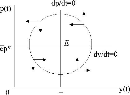
The price level and output motion laws are solutions to the system of
differential equations (1) and (4). One has noticed the similarity between this model
and the famous Predator-prey model. There is a non-trivial stationary point E of
coordinates (y = y, p = ep *). As can be easily observed from the phase diagram

(Figure 1), prices and output display cycles around the equilibrium point. That is,
starting from any other initial point except the stationary point, the price and output
solution belongs to a closed loop (one of the possible paths is depicted in Figure 1,
where the arrows indicate the sense of motion).

^y

Figure 1: the Phase diagram

Let us imagine that policymakers have determined the initial exchange rate e
so that the system is stable, that is, it settles at point E. Unfortunately, any exogenous

<<   7   8   9   10   11   12   13   >>

More intriguing information