IJCSI International Journal of Computer Science Issues, Vol. 4, No. 2, 2009
28
Thus the folklore 1 can be converged in to a theorem as,
Theorem 1: For n records, linear sorting will take a
complexity O (n log n). If the input sequence is presorted,
compared to an unsorted sequence possibly less steps are
sufficient.
Seldom, the theorem does not hold true. It might be the
case that the keys of the objects fall within a known range.
Let there be a controlled environment, where we produce
the keys. For example, we might issue employee numbers
in a given order and in a given sequence, or we might
issue part numbers to items that we manufacture.
Therefore, if the keys are unique and known to be in a
given range, we might allow the key to be the location of
the object (imagine placing the objects in a vector such
that object with key K is in (vector-ref v k)). However the
algorithms presented only rely on the fact that we can
compare keys, to determine if one is less than another
4.2 Folklore 2: In general, we can't sort faster than
O (n log n).
Proof 2: Consider Heap Sort or Bubble Sort or Quick Sort
or Merge Sort or anything else like those, whether already
invented or still to be invented. They all will take at least
O (n log n) steps [5] to sort n items, because of the reason
that, they all work by comparing data items and then
moving data items around based on the outcome of the
comparisons [5]. To illustrate this, here is a piece of Heap
Sort:
If (a[c/2] < a[c]) // if parent is smaller than child
Swap (c/2, c); // trade their values
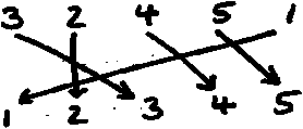
Imagine running such a sort on these numbers:
3, 2, 4, 5, 1
The sort will compare the numbers and based on the
outcomes of that comparison move the values around,
with the net effect of all the moves being summarized by
these arrows:

Fig.1. Suggested moves during swapping process
However it cannot run the same way on same but
differently arranged inputs like 2, 3, 4, 5, 1, as output will
be misleading. Thus the execution must take a different
path for every permutation of inputs.
We can visualize all these executions as an execution tree.
Each node is some action, either an assignment or a
comparison; the tree branches after each comparison; each
path from the root to a leaf is one execution of the
program; and the height of the tree is the (worst-case)
running time of the program. If this is a sorting program
that sorts the numbers 1 through n then execution must
reach a different leaf for each of the n! permutations
of 1....n.
We know that a binary tree with L leaves has height at
least log L where the log is base 2. Thus our execution tree
has height at least log (n!) which is O (n log n).To
conclude, these sorting algorithms must take a different
path of execution for every different permutation of the
input values. There are lots of different permutations (n!).
To be able to run in that many different ways (i.e., for the
execution tree to have that many leaves), the programs
cannot run too quickly (i.e., the execution tree cannot be
too shallow). We may want to conclude that sorting cannot
be done in less than O (n log n) time. This would be an
overstatement because there is a subtle assumption in the
above argument: that the program determines what actions
to take (i.e., how to move values around) solely based on
the outcome of comparisons between the input values. The
lesson learned is, programs that base their actions only on
comparisons of the data cannot beat the O (n log n)
barrier. To have a chance at sorting faster we have to
avoid comparing data! , which is highly impossible.
However, there are situation where we can say that we can
sort faster than O (n log n). For example, Counting Sort
and Radix Sort work faster when the range of values is
limited .Thus the folklore 2 can be converged in to a
theorem as, Theorem 2: For n records, sorting will take
minimum O (n log n) time.
4.3 Folklore 3: The exact number of steps required
by insertion sort is given by the number of inversions
of the sequence
Proof 3: Let a = a0, ..., an-1 be a finite sequence. An
inversion is a pair of index positions, where the elements
of the sequence are out of order. Formally, an inversion is
a pair (i, j), where i < j and ai > aj. Example: Let a = 5, 7,
4, 9, 7. Then, (0, 2) is an inversion, since a0 > a2, namely
5 > 4. Also, (1, 2) is an inversion, since 7 > 4, and (3, 4) is
an inversion, since 9 > 7. There are no other inversions in
this sequence. The inversion sequence v = v0, ..,vn-1 of a
sequence a = a0, ..., an-1 is defined by
Vj = |{ (i, j) | i < j ai > aj }| for j = 0, ..., n-1.
IJCSI
More intriguing information
1. Segmentación en la era de la globalización: ¿Cómo encontrar un segmento nuevo de mercado?2. MANAGEMENT PRACTICES ON VIRGINIA DAIRY FARMS
3. DEMAND FOR MEAT AND FISH PRODUCTS IN KOREA
4. Why unwinding preferences is not the same as liberalisation: the case of sugar
5. Regional differentiation in the Russian federation: A cluster-based typification
6. The name is absent
7. Dendritic Inhibition Enhances Neural Coding Properties
8. Experience, Innovation and Productivity - Empirical Evidence from Italy's Slowdown
9. The name is absent
10. The name is absent