The name is absent

21

(d)

(f)

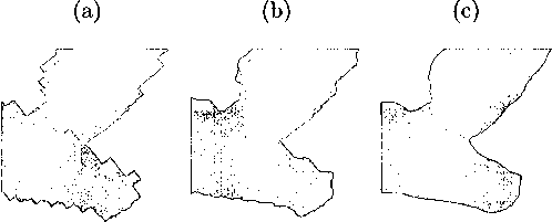
Figure 3.1 : These figures show the result of building scalars from existing segmenta-
tion. The top row of figures is a two-material example, and the bottom four figures
represent the three-material case. 3.1(a) and 3.1(d) are the binary classification
input. 3.1(b) and 3.1(e) are results of assigning all Γs as the scalar field. 3.1(c)
and 3.1(f) are the results of blurring using the heuristic described in Section 3.1.

+/- density map. In the three material case, the contour is formed by the top two
dominant trilinear interpolants (t^fc(τ) and t∙⁷(x)), and Eq. 3.1 is an approximation of
that contour at the voxel x. Figure 3.1 shows the result of our heuristic. We see the
improvement over the arbitrary assignment scheme.

3.2 Importing Iso-surfaces

One standard technique in volume visualization of a function /(ж, у, z) is to create a
piecewise constant transfer function that highlights certain ranges of iso-values [13,
11]. Figure 3.2 shows an example of several nested iso-surfaces visualized in this
manner.

This type of functionality can be reproduced in the multi-material setting in a
natural manner. The basic idea is to import the various volumes bounded by the iso-

<<   28   29   30   31   32   33   34   >>

More intriguing information