Explaining Growth in Dutch Agriculture: Prices, Public R&D, and Technological Change

and Rutten, 1998; cf. Alston, Norton and Pardy (2002) for a similar result for the US). Moreover it
stimulates the development of new innovations, which may partly come from spin-offs of
breakthroughs elsewhere in the Dutch economy or in the international agricultural sphere. As a
consequence the public expenditure on R&D could be well treated as an investment-variable, leading
to the build up of a ‘capital stock’ of innovations and farmer skills. For this reason Figure 1 not only
shows the annual investments in agricultural R&D, but also the accumulated value or the ‘capital
stock’ it creates. It is assumed that new expenditures increase the stock and may have effects lasting
longer than one year. At the same time new investments may create new knowledge and improved
practices, which make part of the old knowledge obsolete. Therefore also a 4% depreciation factor is
applied to the public R&D ‘capital stock’.

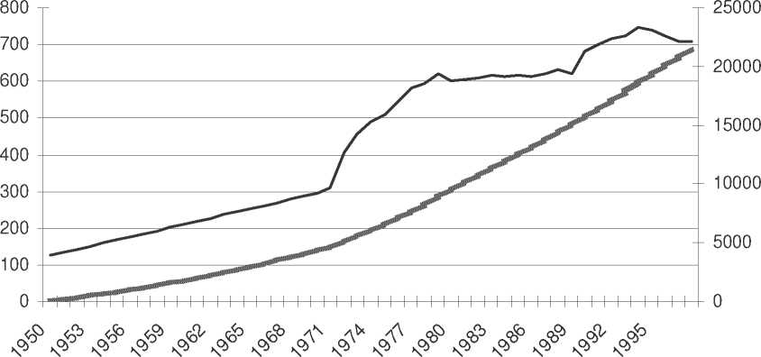
------R&D expenditure                ———— Capital stock

Figure 4 Public R&D expenditures and ‘capital’-formation in Dutch agriculture
Source: Based on Roseboom and Rutten, 1998 and own estimates

Model and specification

Output and input price responsiveness in agriculture has been widely analyzed using a dual
(restricted) profit function approach (Chambers, 1988). The impact of public research expenditures on
agricultural output has been analyzed within the context of a primal production function approach (see
for example Fulginiti and Perrin, 1993). In this study a profit function framework which accounts for
R&D expenditures is chosen.

Following Bouchet et al (1989) let the short-run restricted profit function be ∏ = ∏(P,Z,W) ,
where P is a vector of the expected output and variable input prices (Pi: i=1,...,m), Z is a vector of the
quasi-fixed inputs (Z_j∙: j=1,...,n), and W is a vector of the fixed inputs and exogenous factors. (W_k:
k=1,.,s). Let R be a vector of market prices of the quasi-fixed inputs (Rj: j=1,.n). At a long-run
optimum, the partial derivatives of the restricted profit function with respect to the quantities of the
quasi-fixed inputs (shadow prices) are equal to their long-run equilibrium market prices:

R>=∂∏° ^z∙ ( ^p ■ ^z ■ ⁱ' )

By solving equations (1) for the optimal Zj’s, the long-run, profit maximizing levels of the quasi-
fixed inputs, Z*=Z*(P,R,W) can be derived.

<<   2   3   4   5   6   7   8   >>

More intriguing information