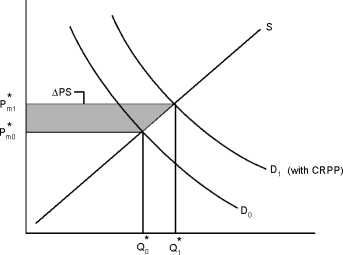
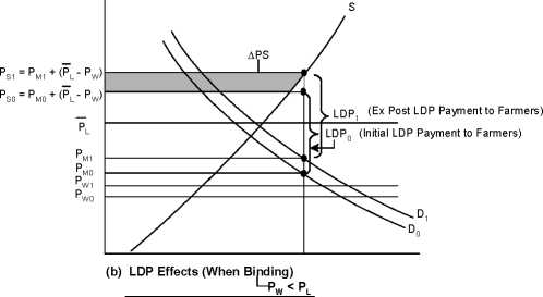
Figure 2. Farm Program Interactions
The influence of U.S. farm programs such as the loan deficiency payment (LDP) system and Step 2 program greatly
complicates the calculation of Return on Investment (ROI).

(a) Free Market: No Program Effects From LDP or STEP 2
Here Pm* = Market Price = Supplier Price = Demand Price
∆PS = Producer Benefits from Demand Shift

PM = Market Price = Demand Price
PS = PM + (PL - PW) = Supply Price
PW = World Price, where PW = F (PM)
PL = LDP Rate (Fixed)
(Shift effects on producer price:)
∆PS = (PS1 - PS0) = (PM1 - PM0) - (PW1 - PW0) = ∆PM - ∆PW
Since ∆PW > 0, then ∆PS < ∆PM (Also LDP1, < LDP0)
Calculate ∆PS accordingly

(c) Step 2 Program Effects
Pm = Market Price = Supply Price
PW = World Price = Demand Price (Demanders are guaranteed
to pay world price + $0.0125)
(Shift Effects)
∆PM is larger than it would be in a free market (∆PM*)
∆Q is larger than it would be in a free market (∆Q*)
(d) Combined Effects of LDP & Step 2
Ps = Supply Price = Pm & (p_ - Pw)
PW = Demand Price = World Price (Guaranteed + $0.0125—not depicted)
PM = "Market" Price, though it is neither a supply nor a demand price
PM* = Free market price
(Shift Effects)
∆PS < ∆PM, but ∆PM vs ∆PM* is an empirical issue
Panel (b) introduces the effects of the LDP system. If the adjusted world price (AWP) of cotton
falls below the loan rate of 51.92 cents per pound, cotton growers are eligible for a supplemental payment
equal to the difference between the loan rate and the AWP. The total price received by the grower is
equal to the price they receive in the market (Pm) plus the supplemental payment (-l - Pw), where -l is
the loan rate and PW is the AWP. The demand shift raises the U.S. market price from PM0 to PM1.
However, the total price to suppliers will be less than PM1 if the loan rate is binding and the rise in the
11
More intriguing information
1. Financial Development and Sectoral Output Growth in 19th Century Germany2. Managing Human Resources in Higher Education: The Implications of a Diversifying Workforce
3. The name is absent
4. The name is absent
5. Deprivation Analysis in Declining Inner City Residential Areas: A Case Study From Izmir, Turkey.
6. The name is absent
7. Tourism in Rural Areas and Regional Development Planning
8. Firm Creation, Firm Evolution and Clusters in Chile’s Dynamic Wine Sector: Evidence from the Colchagua and Casablanca Regions
9. Structural Breakpoints in Volatility in International Markets
10. The name is absent