26
Stata Technical Bulletin
STB-4
computer for weeks. The value of such work lies in the possibility of finding applications where bootstrapping solves (or less
gratifyingly, fails to solve) otherwise intractable problems.
Notes
1. X represents population density in people per square mile. Y represents metric tons of NOx emissions per square mile. The more crowded (also
poorer) areas are, of course, more polluted.
2. The mean bootstrap slope estimates are given.
3. Bootstrap standard errors are standard deviations of the bootstrap distributions; original-sample SE is that printed by regress.
References
Efron, B. and R. Tibshirani. 1986. Bootstrap methods for standard errors, confidence intervals, and other measures of statistical accuracy. Statistical
Science 1(1): 54-77.
Hall, P. 1988. Theoretical comparison of bootstrap confidence intervals. The Annals of Statistics 16(3): 927-953.
Hamilton, L. C. 1991a. ssi1: Monte carlo simulation. Stata Technical Bulletin 1: 25-28.
——. 1991b. srd1: How robust is robust regression? Stata Technical Bulletin 2: 21-26.
——. 1992. Regression with Graphics: A Second Course in Applied Statistics. Pacific Grove, CA: Brooks/Cole.
Stine, R. 1990. An introduction to bootstrap methods: examples and ideas. In Modern Methods of Data Analysis, ed. J. Fox and J. S. Long, 353-373.
Newbury Park, CA: Sage Publications.
Zupan, J. M. 1973. The Distribution of Air Quality in the New York Region. Baltimore: Johns Hopkins University Press.

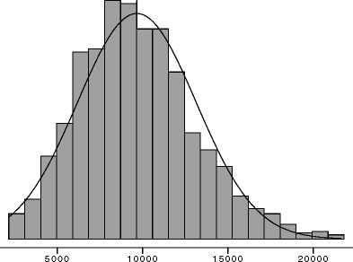
Figure 1: Means from 1,000 bootstrap samples
data resampling
s = 21.0*10^-7

5.0e-06 .00001 .000015 .00002 .000025

Figure 2: Regression slopes from 1,000 bootstrap samples
Figure 1
Figure 2
Y

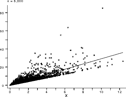
Figure 3: A problematic regression--model [7]
Figure 3

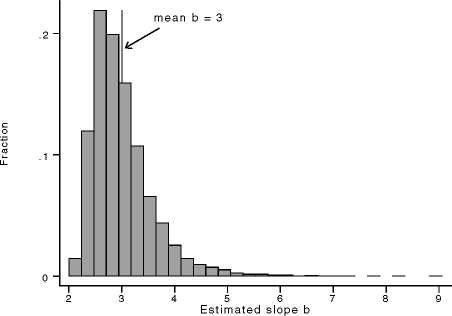
Figure 4: 10,000 n=80 Monte Carlo samples, model [7]
Figure 4
More intriguing information
1. The name is absent2. Quality Enhancement for E-Learning Courses: The Role of Student Feedback
3. The name is absent
4. The name is absent
5. Keynesian Dynamics and the Wage-Price Spiral:Estimating a Baseline Disequilibrium Approach
6. The name is absent
7. Sector Switching: An Unexplored Dimension of Firm Dynamics in Developing Countries
8. The name is absent
9. THE USE OF EXTRANEOUS INFORMATION IN THE DEVELOPMENT OF A POLICY SIMULATION MODEL
10. Beyond Networks? A brief response to ‘Which networks matter in education governance?’