The Impact of Optimal Tariffs and Taxes on Agglomeration

The real wage relation can be determined now easily and is given by:
wr_ σγ [P^1-σTΘ* + P*^1-σT*] + γ² (1 - L) [ΘΘ* -1] P*y(1 — TA)1-γ
wR = σγ ∣ΘP*^1-σT* + P ^1-σT^] + γ²L [ΘΘ* - 1] × P^γ(1 — TA)^1-γ (
where the last term denotes the relative regional price level.

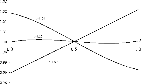
As a reference case, figure 1 presents the real wage relation of (10) if pol-
icy is inactive (TI =T_I^* =TI =T_I^* =0). In all cases the real wage relation gets
unity at L = 0.5 indicating that the symmetric equilibrium is also a long-
run equilibrium. But, the stability of this long-run equilibrium depends on
the real wage relation in case of small disturbances. Consider for instance
a labor share slightly above 0.5 in one region as in the case of τ = 1.02.
Since this deviation of the symmetric equilibrium implies a short-run wage
relation above unity even more firms and skilled migrates to this region. Ag-
glomeration occurs and the symmetric equilibrium is unstable. Technically,
the symmetric equilibrium is unstable if the slope of the corresponding real
wage curve is positive. The critical trade cost level, below which instability
of the symmetric equilibrium occurs, is usually called ’breakpoint’.

Parameters: γ = 0.5, σ = 4

Figure 1: Domestic real wage relation and skilled labor share

If the symmetric equilibrium is unstable other stable long-run equilibria
must exist with agglomeration in one of the two regions. If, like in the

<<   9   10   11   12   13   14   15   >>

More intriguing information