Labour Market Flexibility and Regional Unemployment Rate Dynamics: Spain (1980-1995)

Next, we introduce a one-off unit labour demand shock at period t = 0, i.e. ε_iⁿ₀ = 1,
ε_iⁿ_t = 0 for t ≥ 1, in each of the regional panel models. The generated unemployment
rate impulse response functions for both regional groups are plotted in Figure 3a. To
get a perspective of the temporal persistence of the shocks and compare the resulting
trajectories, the impulse response functions in Figure 3 have been normalised so that the
immediate impact of the shock is unity. The responses through time of the unemployment
rate to a unit one-period wage setting and labour supply shocks are presented in Figure
3b and 3c, respectively.

Figure 3. Impulse response function of unemployment to a temporary shock

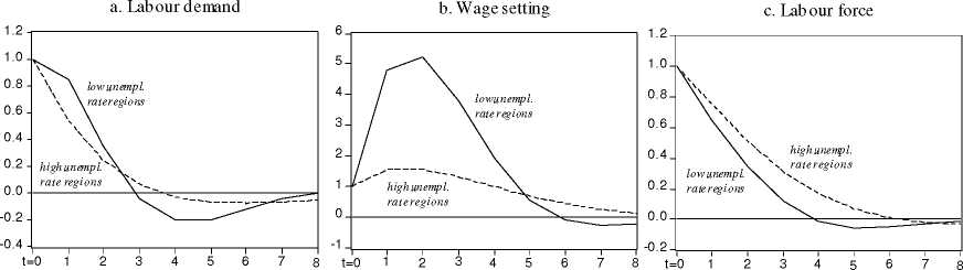
Responses of unemployment to a one-off unit shock ocurιing at period t=0. The responses have been normalized so that the inmediate impact is unity

Figures 3a and 3c show that the unemployment effects of labour demand and supply
shocks start decreasing once the shock has been initiated. In contrast, Figure 3b shows
that the real wage shock continues to push up unemployment for another two years after
its initial impact before it starts to gradually dissipate. This pattern is more profound in
the high unemployment group of regions than in the low unemployment group.

It takes several years before the one-off shocks are completely absorbed by the labour
market. In particular, 20% of the initial impact of the shock is still felt by the market
after approximately two years (labour demand shock), or five years (wage shock), or three
years (labour supply shock).

It is also useful to examine the propagation mechanisms from a quantitative perspec-
tive. For each shock, we calculate unemployment persistence (σ) by substituting the
respective impulse response function in equation (11). In other words, unemployment
persistence is the sum of all the after-effects of the shock.

The total effect (τ ) of the shock on unemployment is obtained by simply adding the
"current" effect, i.e. the initial unemployment response (R₀), to the "future" effect, i.e.
∞

the persistense measure: τ ≡   Rt = R0 + σ. It is important to note the following distinc-

t=0

tion. While the size of the shock should be understood as the instantaneous direct effect
that it has on the dependend variable, the initial response captures both the direct and
indirect effects of the shock on unemployment. The indirect effects are due to spillovers.
When there are no spillover effects in the labour market system, the initial unemployment

17

<<   14   15   16   17   18   19   20   >>

More intriguing information