Labour Market Flexibility and Regional Unemployment Rate Dynamics: Spain (1980-1995)

rate is trendless in the long-run. In general, equilibrating mechanisms in the labour market
and other markets are jointly responsible for this phenomenon. Thus restrictions on the
relationships between the long-run growth rates (as opposed to the levels) of capital stock
and other growing exogenous variables are sufficient for this purpose.

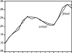
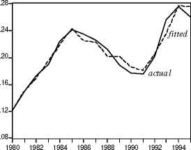
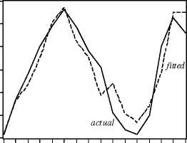
Figure 2 shows that the fitted unemployment rate generated by our system tracks the
trajectory of the actual unemployment rate very accurately.

In the following sections we seek to examine the role played by the lagged adjustment
processes and their interplay with the changes in the exogenous variables in the evolution
of the unemployment rate.

a. High unemployment regions

1980 1982 1984 1986 1988 1990 1992 1994

c. Aggregate unemployment rate

Figure 2. Actual and fitted values

b. Low unemployment regions

1980 1982 1984 1986 1988 1990 1992 1994

.24

.22

.20

.18

.16

.14

.12

5 Persistence of Shocks

We first show that the set of lagged adjustment processes in the model and their interplay
with the feedback mechanisms give rise to the propagation of shocks. In the context of
the estimated models in Tables 5 and 6, we measure the impacts of the different labour
market shocks on the time path of the unemployment rate for the two groups of regions.

Following the methodology outlined in section 2, we derive the reduced form unem-
ployment rate equation for each group of regions

ρ (L) u_it = b (L) x_it + c (L) z_t + θ_d (L) ε_iⁿ_t + θ_w (L) ε_i^w_t + θ_s (L) ε^l_it,          (18)

where the autoregressive polynomial ρ (L) is dynamically stable,³⁶ xi_t is a 3 × 1 vector
of exogenous regional variables and z_t is a 4 × 1 vector of exogenous national variables;
b (L) and c (L) are 1 × 3 and 1 × 4 vectors of lag polynomials, respectively; ε_iⁿ_t , ε_i^w_t , and ε^l_it
are the error terms in the labour demand (employment), wage setting, and labour supply
(labour force) equations, respectively, given in Tables 5-6. Note that the parameters in all
of the above lag polynomials - autoregressive ρ (∙), slope b (∙), c (∙), and moving average
θ (∙) - are functions of the estimated coefficients given in Tables 5-6.

³⁶ Note that ρ₀ = 1 so that ρ (L) = 1 + ρ₁L + ... + ρ_qL^q. Dynamic stability implies that the roots of
ρ (L) = 0 lie outside the unit circle.

16

<<   13   14   15   16   17   18   19   >>

More intriguing information