Handling the measurement error problem by means of panel data: Moment methods applied on firm data

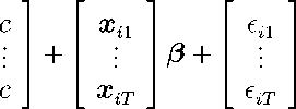
may be due to lagged response, autocorrelated measurement errors or disturbances
and/or (deterministic or stochastic) trends in the capital input relationship. The
latter would violate, for example, the stationarity assumption for capital. Owing to
the short time span of our data, we have not, however, performed a cointegration
analysis.

All the results in Table 24.2 uniformly indicate a marginal input elasticity of
materials, 1 /μ, larger than one ; β Dx and β Dx are, however, lower than the (in-
consistent) estimate obtained by running OLS regression on differences (cf. β^b _OLSD
for the materials-output regression in Table 24.1), and β^b_Dy and βe _Dy are higher
than the (inconsistent) estimate obtained by running reverse OLS regression on
differences (cf. β^b _OLSD for the output-materials regression in Table 24.1).

Equation in levels, IV’s in differences. We next consider the procedures for
estimating all the level equations (3) with the IV’s in differences. The T stacked
level equations for individual i are

^yi1

.

.

.

y_iT

or compactly, omitting the ‘dot’ subscript [cf. (4)],

y_i =e_Tc+X_iβ+_i.

The IV matrix (cf. Proposition 2) is the (T × T (T - 2)K) matrix

^δ xi (1) ∙∙∙     0

^..                      ^..                          ^..

_.                             ._.

0     ∙∙∙  ∆x_i(T)

Again, we use different IV’s for different equations, considering (44) as T equations
with β as a common slope coefficient. Let

y =[y₁⁰,...,y_N⁰ ]⁰,         =[₁⁰,...,_N⁰ ]⁰,

X =[X1⁰,...,XN⁰ ]⁰, ∆Z= [(∆Z1)⁰,...,(∆ZN)⁰]⁰.

23

<<   21   22   23   24   25   26   27   >>

More intriguing information