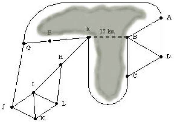
FIGURE 7: A system subject to
change
Figure? shows a numerical simulation
of the case above. For the purpose of
illustration, we show a case with a 1-
dimensional geography, i.e., we
assume that all the population is
located along the same road. The
position is measured in terms of the
distance to CBD1, while CBD2 is
located at a distance dCBD from CBD1.
It is straightforward to extend (4.2) to the general case. If there are 3 CBDs in the system, we put
(4.3)
R[di, d2,d3] = D(d1) D(d2) D(d2)Rx
+(1 - D(di))D(d2)D(d3)R⅞[d1]
+(1 - D(d2))D(d)D(d3)R[d1]
+(1 - D(d3))D(d1)D(d2)R3[d1]
+(1 - D(d1))(1 - D(d2)) D(d3) R12 [(d1 + d2) /2]
+(1 - D(d1))(1 - D(d5)) D(d2) R13[(d + d3)/2]
+(1 - D(d2))(1 - D(d3)) D(d1) R23[(d2 + d3) /2]
+(1 - D(d1))(1 - D(d2))(1 - D(d3))Rk3[(d1 + d2 + d3)/3]
Expression (4.3) then defines E/L in terms of a convex combination of the 8 states
R8,R1,R2,R3,R12,R13,R23, and R123. The extension to the general case with N CBDs follows similarly.
Note that the number of states in the model will increase exponentially with N. This, however, is not
a problem since we will always expect that the total number of CBDs is quite small.
5. Empirical results from the model
In preparation.
6. Concluding remarks
In preparation.
REFERENCES
Anas, A. 1987. Modeling in Urban and Regional Economics, Fundamentals of pure and applied
economics, 26, Harwood academic publishers.
14
More intriguing information
1. The name is absent2. The name is absent
3. The name is absent
4. The name is absent
5. The name is absent
6. Fertility in Developing Countries
7. Handling the measurement error problem by means of panel data: Moment methods applied on firm data
8. The name is absent
9. The name is absent
10. PROJECTED COSTS FOR SELECTED LOUISIANA VEGETABLE CROPS - 1997 SEASON