Fig. 3: Commuting rate by employment density (spatial categories, NUTS 3)
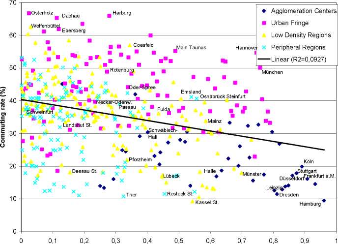
Employment density (GINI-Coefficient)
Source: Employment statistic 2003.
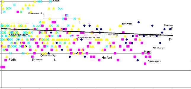
Fig. 4: Average commuting distance by employment density (spatial categories,
NUTS 3)
50
Agglomeration Centers
Frankfurt (Oder)
Kiel
45
40
35
ɪ
φ
30
га
ω
□
25
20
15
10
Bremerhaven
Urban Fringe
Low Density Regions
Landshut, St.
Brandenburg, KS
Lübeck
X
Peripheral Regions
—Regensburg, St.------
X Magdeburg, St.
R2=0,0087
Linear (R2=0,0087)
Koblenz
Ulm
X
X AX X
+____^Dresden
Leipzig
Cottbus
X X
× Trier
Jena, St.
FuldaBKleve
××
Borken
К ХЖ XB > X
Herford
München
Oberallgau
Erlangen-Hochst.
Г >Cf × Ж
X XX
⅜ ichwabisch-H⅛n—Emsland
Frankfurt a.M.
0,1 0,2
0,3 0,4 0,5 0,6 0,7 0,8 0,9
×Passau, St.
Düsseldorf
Koln «
Hamburg
Stuttgart München, St
nover_______________________
Employment density (GINI-Coefficient)
Source: Employment statistic 2003.
17
More intriguing information
1. The name is absent2. Orientation discrimination in WS 2
3. The name is absent
4. Fertility in Developing Countries
5. The ultimate determinants of central bank independence
6. The name is absent
7. Does Market Concentration Promote or Reduce New Product Introductions? Evidence from US Food Industry
8. The name is absent
9. Computational Experiments with the Fuzzy Love and Romance
10. PROTECTING CONTRACT GROWERS OF BROILER CHICKEN INDUSTRY