Evolution of cognitive function via redeployment of brain areas

to BL activations, and I matched RL activations in an area to other RL activations of that
area, as well as to BL activations. I followed the same procedure for medial activations.

I did not match bilateral activations to each other.

To calculate the diversity of activations across task categories I employed a standard
measure of population diversity, Diversity Variability (DV). DV is calculated using the
following equation, a version of standard deviation, where Cati is the proportion of
activations in category i; mean is the mean proportion of activations in each category
(always 0.25 for 4 categories), and k is the number of categories:

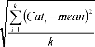
The category diversity of a given area is just (1-DV). With four categories, category
diversity ranges from 0.57 (all items in one category) to 1 (equal numbers in each
category). Note that for the purpose of calculating category diversity, the activation
counts in each category were normalized to n=42.

Finally, to measure the distribution, or “scatter” of areas activated by a given task, I
constructed an adjacency graph for the cortex (Figure 3). A graph is a set of objects
called points or vertices connected by links called lines or edges. For constructing a
graph of the cortex, I took the nodes to be numbered Brodmann areas (Brodmann, 1907)
and the edges to indicate adjacency. Adjacency in this context means only that the
Brodmann areas share a physical border in the brain.

<<   3   4   5   6   7   8   9   >>

More intriguing information