The name is absent

(a)

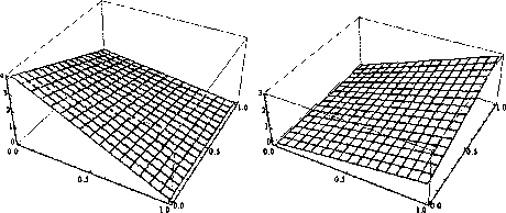
Figure 2.2 : 2 material example continued. 2.2(a) is the plot of the function in 2.1 by
replacing the negative voxels (coefficients of the bilinear) with O’s. 2.2(b) is the plot
of the same function by replacing the positive voxels with O’s and taking the absolute
value of the coefficients. 2.2(c) is the maximum of the functions in 2.2(a) and 2.2(b).

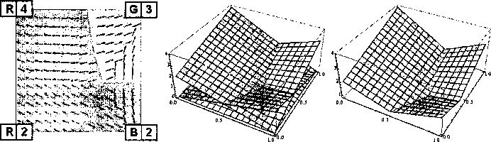
Figure 2.3 : 3 material example. 2.3(a) is the classification of the bi-linear function
under our scheme. The arrows denote the gradient. 2.3(b) is the plot of 3 functions
that are created under our evaluation scheme. 2.3(c) is the maximum plot of the
three functions.

ure 2.1(b) shows the associated bi-linear s(x) interpolant partition into positive and
negative regions. Figure 2.2 illustrates our classification method on this example. Fig-
ures 2.2(a) and 2.2(b) shows the functions t⁺(x) and t~(x), respectively. Figure 2.2(c)
shows a plot of the maximum of these two functions. Note that the partition of the
pixel in figures 2.1(b) and 2.2(c) are equivalent.

Figure 2.3(a) shows another 2D example in which the four corners of the pixel
have three distinct materials, red, green and blue. Figure 2.3(b) show plots of the
three bi-linear functions associated with the materials. Finally, Figure 2.3(c) shows a

<<   19   20   21   22   23   24   25   >>

More intriguing information