Optimal Tax Policy when Firms are Internationally Mobile

As a benchmark case, consider first the optimal tax policy with respect to the
tax rate and the tax base when firms are immobile.

3.4 Optimal tax policy with immobile firms

With A^h > A⁺, the welfare function becomes

W = U ^j У [F (1 - u) - (1 - au) K] dAdB^ +H ^j ʃ и (F

with F = F (K, A, B) for simplicity, subject to

F(K,A^l) (1 - и) - (1 - au) K = 0                 (19)

for every given level of B. Figure 1 shows the two-dimensional profitability
space of the firms in the economy:

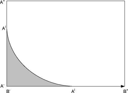
Figure 1: Immobile firms.

The firms in the shaded left bottom corner are not profitable enough and do not
produce. Firms in the white area do produce and can be taxed. Firms along the A^l
frontier are indifferent between producing and leaving the market. By increasing
(lowering) the effective tax burden, the government shifts the A^l frontier to the
lower left (upper right).

The optimality conditions with respect to u and a are:

10

<<   9   10   11   12   13   14   15   >>

More intriguing information