30

Value of the multiplier
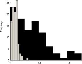
Figure 2: Histograms of average (grey) and dynamic (black) multiplier with a
random network of monetary transactions.
We then consider one single economy with a fixed set of parameters (thus
fixing the average multiplier) and simulate 1000 different processes of money
creation by randomly inject money on different sites. Fig. 3 shows the empirical
cdf of the resulting dynamic multiplier: as it can be seen, the monetary system
is path dependent and the final size of the money multiplier depends, among
other things, on the position where money is injected into the economy. This
means that the multiplier could change even when behavioural ratios for banks’
reserves and households’ currency remain fixed, an aspect that is completely
neglected by the standard theory.
The next topology that we consider is a regular structure, where banks and
households are laid down on a bi-dimensional lattice. Each bank is linked to four
households, and each household to four banks. Each link is bi-directional, for
deposits and loans (though some can have zero weight). We simulate the process
of money creation on a lattice composed by 18 banks and 18 households, and
show the distribution (histograms) for the average and the dynamic multipliers
in Fig. 4. Compared with the case of a random graph, the variability in the
dynamic multiplier is now reduced, as the presence of absorbing states does not
disconnect entire regions of the system.
To conclude, we look at the extreme case of a star topology, where all house-
holds are linked to one single bank which receives deposits and extends loans
to them. We simulate the process of money creation on a structure of this type
with 100 households and one bank, and show the results in Fig.5. As we can
see, the variability in the dynamic multiplier increases again now, because the
presence of only one bank makes the whole system dependent on the behaviour
of that bank.
More intriguing information
1. Short Term Memory May Be the Depletion of the Readily Releasable Pool of Presynaptic Neurotransmitter Vesicles2. ASSESSMENT OF MARKET RISK IN HOG PRODUCTION USING VALUE-AT-RISK AND EXTREME VALUE THEORY
3. Centre for Longitudinal Studies
4. The name is absent
5. The name is absent
6. Should Local Public Employment Services be Merged with the Local Social Benefit Administrations?
7. The name is absent
8. Langfristige Wachstumsaussichten der ukrainischen Wirtschaft : Potenziale und Barrieren
9. Sector Switching: An Unexplored Dimension of Firm Dynamics in Developing Countries
10. What Contribution Can Residential Field Courses Make to the Education of 11-14 Year-olds?