Stable Distributions

1.5 Estimation of parameters

Sample of size N=10^4

-4           -2           0            2            4

log(x)

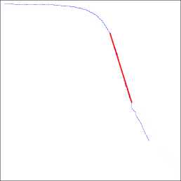
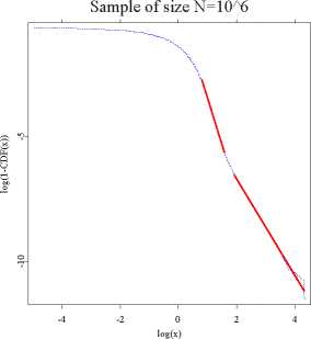
Figure 1.4: A double logarithmic plot of the right tail of an empirical symmetric
1.9-stable distribution function for a sample of size N = 10⁴ (left
panel) and N = 10⁶ (right panel). Thick red lines represent the
linear regression fit. The tail index estimate (<^ = 3.7320) obtained
for the smaller sample is close to the initial power-law like decay of
the larger sample (<^ = 3.7881). The far tail estimate α = 1.9309 is
close to the true value of α.

θ STFstab04.xpl

i.e. the negative tail) observations, after a crossover from a temporary power-
like decay (which surprisingly indicates α ≈ 3.7). Moreover, the obtained
estimates still have a slight positive bias, which suggests that perhaps even
larger samples than 10⁶ observations should be used. In Figure 1.4 we used
only the upper 0.15% of the records to estimate the true tail exponent. In
general, the choice of the observations used in the regression is subjective and
can yield large estimation errors, a fact which is often neglected in the literature.

A well known method for estimating the tail index that does not assume a
parametric form for the entire distribution function, but focuses only on the
tail behavior was proposed by Hill (1975). The Hill estimator is used to estimate
the tail index α, when the upper (or lower) tail of the distribution is of the
form: 1 - F (x) = Cx^-α, see Figure 1.5. Like the log-log regression method, the
Hill estimator tends to overestimate the tail exponent of the stable distribution

<<   9   10   11   12   13   14   15   >>

More intriguing information