The name is absent

and that VT₁,₃(x,y) = (2.27; 4.84; 6.86) and VT₃,2(x,y) = (2.46; 4.58; 6.92) are not LD-comparable,
although labor and capital tax schedules are separately comparable by ψ(x) and ψ(y), and
also using the Lorenz Domination criterium. Although income distribution of this example is
not dense, we obtain exactly what Jakobbson (1976) predicts (see Calonge and Tejada, 2009,
for a further argument on how density of can affect Jakobsson results).

In conclusion, if Condition 1 does not hold, dual tax cuts T1,3 and T3,2 cannot be compared,
neither by ψ(x+y) nor ψ (x,y) nor using the Lorenz Domination criterium on the total post-
tax income distribution, as it is the case when such condition does hold. Therefore, Condition
1 is necessary. Similar examples show that Condition 2 also necessary.

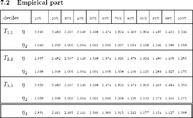
Table A.3. Losers and gainers analysis: elasticities.

References

[1] Arcarons, J., Calonge, S. (2004). ”Modelo de Microsimulacion SIMESP v4.0 (O® B-
3916-08”. e-publica.

35

<<   33   34   35   36   37   38   39   >>

More intriguing information