The name is absent

c) Negative feedback with variable information delay

If we assume that information delay time is variable, as a function of the total flux (F = W_c + W_w) and of the volume
of the pipe from the mixer to the sprinkler (Vo), we can calculate the time the mixed water needs to reach the sprinkler by the
equation dly = V./F.

Now, we replace the parameter dly in line 16 with two auxiliary equations

. replace _model="A F=Wc+Ww^,' in 16

. replace _model=”A dly=Vo∕F^,' in 17

and we assign the value to the parameter Vq by the line:

. replace _model=”P Vo=O. 6” in 18

Thus, it is possible to simulate the warm water flux and the mixed water temperature with a variable information delay by typing
‘simula, dt(0.2) tspan(12)’. The simulation results are shown in Figure 6(c).

d) Negative feedback with variable material delay

A different pattern of water regulation is still obtained if we consider a variable material delay. In this case the delayed
quantity is not lost but is cumulated to the other delayed quantity. This could be the case when a lizard is taking a shower. It is
not warm-blooded and then we can suppose its reaction time depending on the water temperature. Even if the very mixed water
temperature is perceived without information delay, the regulation performed by the lizard is very slow at low temperature and
fast at high temperature. Anyhow, the regulation quantity is not forgotten by the lizard but only delayed and maybe cumulated
if the delay time is shortening with time. In this situation the dynamic of the water flux regulation can be complex and shown
in Figure 6(d), for a time reaction coefficient of R_tc = 0.05. To obtain a variable material delay, .model is modified by

. replace _model=”R VAw=MDL[K*(Topt-T) ,dly] ^,, in 7

. replace _-model="A dly=Rtc*T^,' in 16

. replace _-model="P Rtc=O.05” in 17

. drop in 18

. simula, dt(0.2) tspan(12)

The previous example with variable material delay is not completely pertinent. A better example could be the arrival rate
of wares in a harbor, transported by ships. If further goods are needed (system state) the information requiring other goods is
quite without retard in respect to the material delay due to the time for transport. If the ships have different speeds, the material
delay is variable, and it is possible that ships starting at different times arrive at the destination on the same day. In this case
the wares are not lost but are cumulated for all the ships arriving on the same day.

Figures

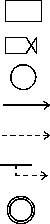
State variable (integral of the rates)

Rate variable (material flow)

Auxiliary variable

Material flow and direction

Information links (flow and direction)

Constant or parameter

Exogenous variable

prey              predator

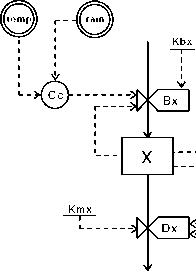
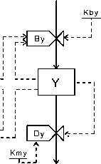
Figure 2

Figure 1 shows the graphic symbols for the relational diagram of the system. Figure 2 shows the relational diagram by the Forrester (1968) conventions
of the prey-predator interaction in a “Volterra model.” The state variables are X (prey density) and Y (predator density). Bx, By, Dx, Dy represent,
respectively, the birth and mortality rates for prey and predator. Cc is the “carrying capacity” of the ecosystem. (Both graphs were drawn “freehand”
using Stage.)

<<   27   28   29   30   31   32   >>

More intriguing information