The name is absent

Stata Technical Bulletin

Options

grid adds grid lines at the 0.25, 0.50, 0.75 quantiles and also, in the case of qsm and qdagum, at the 0.05, 0.10, 0.90, and 0.95
quantiles.

graph-options are any of the options allowed with graph, twoway; see help for graph.

Description

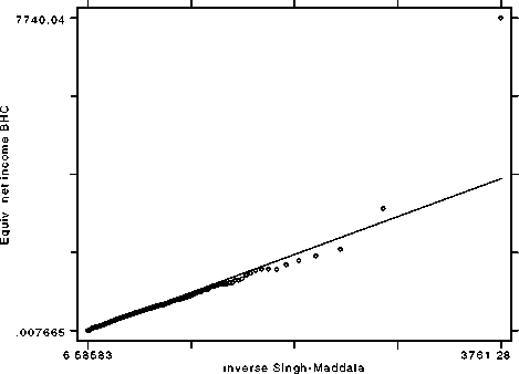
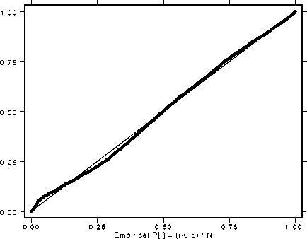
psm produces a probability plot for varname compared with a three-parameter Singh-Maddala distribution. qsm plots the
quantiles of varname against the quantiles of a three-parameter Singh-Maddala distribution. The parameters a, b and q are taken
from global macros S_a, S_b, and S_q, which is where smfit puts maximum likelihood estimates of them.

pdagum produces a probability plot for varname compared with a three-parameter Dagum distribution. qdagum plots the
quantiles of varname against the quantiles of a three-parameter Dagum distribution. The parameters b, d and ∕ι are taken from
S_b, S_d, and S_h, which is where dagumfit puts maximum likelihood estimates of them.

smfit and dagumfit are discussed in Jenkins (1999b).

Example

The illustrative example uses the same income distribution data as described in Jenkins (1999a). The income variable is
eybhc with fweight variable wgt.

Singh-Maddala and Dagum distributions were first fitted using smfit and dagumfit (as in Jenkins 1999a), except that
grossing-up weights were neglected this time since the plotting programs do not handle them. The results are as follows:

. smfit eybhc if eybhc >0

(output omitted )

. qsm eybhc if eybhc>0, SavingCqsml.gph,replace)

. psm eybhc if eybhc>0, SavingCpsml.gph,replace)

. dagumfit eybhc

(output omitted)

. qdagum eybhc if eybhc>0, savingCqdaguml.gph,replace)

. pdagum eybhc if eybhc>0, SavingCpdaguml.gph,replace)

. graph using psml pdaguml qsml qdaguml

Figure 1. Output from qsm

Figure 2. Output from psm

<<   1   2   3   4   5   6   >>

More intriguing information