The name is absent

pred

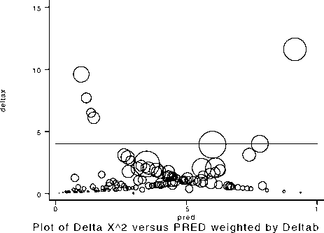
Plot of Delta X^2 versus PRED

Figure 1

Figure 2

References

Hamilton, L. C. 1992. Regression with Graphics. Pacific Grove, CA: Brooks/Cole Publishing Company.

Hosmer, D. W. and S. Lemeshow. 1989. Applied Logistic Regression. New York: John Wiley & Sons.

ssi2 Bootstrap programming

Lawrence C. Hamilton, Dept. of Sociology, University of New Hampshire

Bootstrapping refers to a process of repeatedly sampling (with replacement) from the data at hand. Instead of trusting theory
to tell us about the sampling distribution of an estimator b, we approximate that distribution empirically. Drawing B bootstrap
samples of size n (from an original sample also size n) obtains B new estimates, each denoted b*. The bootstrap distribution
of b* forms a basis for standard errors or confidence intervals (Efron and Tibshirani, 1986; for an introduction see Stine in Fox
and Long, 1990). This empirical approach seems most attractive in situations where the estimator is theoretically intractable, or
where the usual theory rests on untenable assumptions.

Bootstrapping requires fewer assumptions but more computing than classical methods. The January 1991 Stata News (p.6-7)
described two general bootstrap programs, bootsamp.ado and boot.ado. Help files document these programs, which provide
a relatively easy way to start bootstrapping. Even with these ready-made programs, however, users must do some programming
themselves and know exactly what they want. This can be tricky: bootstrapping is fraught with nonobvious choices and with
“obvious” solutions that don’t work. Researchers have the best chance of successful bootstrapping when they can write programs
to fit specific analytical needs. Towards this goal I reinvent the wheel below, showing the construction of several simple bootstrap
programs. Rather than being general-purpose routines like boot. ado or bootsamp. ado, these four examples are problem-specific
but illustrate a general, readily modified approach.

The first three examples expect to find raw data in a file named source.dta, with variables called X and Y. For illustration
I employ data from Zupan, 1973, on the population density (X) and air pollution levels (Y) in 21 New York counties:¹

<<   <   15   16   17   18   19   20   21   >   >>