45
Stata Technical Bulletin
43
mpg

ooooooooooo
ooooooooo
oooooooo
O O
OOOOOO
O O
-16
9 -
-10
1o^
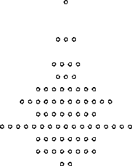
Figure 1. A simple turnip plot for mpg for the auto data.
Figure 2. Higher resolution graph for mpg with line at median.
Finally, we do a turnip plot for only foreign cars with a specified ж-axis label and a horizontal line at the mean.
. turnip mpg if foreign==!, xlabel(-10 10) yline(mean)
# of observations per turnip row is the frequency below:
|
≡pg I |
Freq. |
Percent |
Cum. |
|
— | |||
|
13.88521 I |
1 |
4.55 |
4.55 |
|
16.19941 I |
2 |
9.09 |
13.64 |
|
18.51361 I |
2 |
9.09 |
22.73 |
|
20.82781 I |
2 |
9.09 |
31.82 |
|
23.14201 I |
4 |
18.18 |
50.00 |
|
25.45621 I |
5 |
22.73 |
72.73 |
|
27.77042 I |
1 |
4.55 |
77.27 |
|
30.08462 I |
2 |
9.09 |
86.36 |
|
34.71302 I |
2 |
9.09 |
95.45 |
|
41.65562 I |
1 |
4.55 |
100.00 |
|
— | |||
|
Total I |
22 |
100.00 |
options: XlabeK-IO 10) yline(24.7) ylabel( 24.77272727272727 11 44 )
resolution: 2.314201283894056
yline: 24.77272727272727 (mean)
This gives the plot in Figure 3.
44 -
σ>
E
24.7727
11
h-
-10
Figure 3. Turnip plot for foreign cars with specified я-axis label and a horizontal line at the mean.
More intriguing information
1. Educational Inequalities Among School Leavers in Ireland 1979-19942. Modelling the Effects of Public Support to Small Firms in the UK - Paradise Gained?
3. Testing Hypotheses in an I(2) Model with Applications to the Persistent Long Swings in the Dmk/$ Rate
4. The name is absent
5. Placentophagia in Nonpregnant Nulliparous Mice: A Genetic Investigation1
6. Non-causality in Bivariate Binary Panel Data
7. Announcement effects of convertible bond loans versus warrant-bond loans: An empirical analysis for the Dutch market
8. The name is absent
9. Evidence-Based Professional Development of Science Teachers in Two Countries
10. The purpose of this paper is to report on the 2008 inaugural Equal Opportunities Conference held at the University of East Anglia, Norwich