A production model and maintenance planning model for the process industry

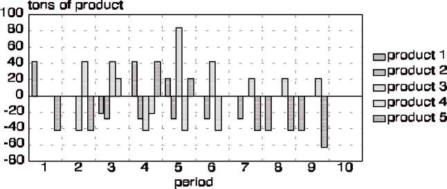
Figure 3: Inventories and backorders for the basic scenario

	Basic scenario	Scenario 1	Scenario 2	Scenario 3
Setup costs	sij=1,000 for all i,j	sij=3,000 for all j si_j=1,000 for i=2,...,5, j=1,2________________	s_ij=1,000 for all i,j	sij=1,000 for all i,j
Capacity	Capj=336 for all j	Capj=336 for all j	Cap₁=336 Cap₂=168	Capj=336 for all j
Backorder costs	l_i=1,000 for all i	l_i=1,000 for all i	l_i=1,000 for all i	l₁=3,000 l_i=1,000 for i=2,...,5

Table 6: Summary of the four scenarios

	Job sequence	Objective value ($)
Scenario 1	Line 1: 1 2 3 1 2 M 2 2 1 1 Line 2: 4 4 5 5 3 M 4 5 3 5	285,620
Scenario 2	Line 1: 4 4 5 1 M 5 2 1 1 4 Line 2: 4 3 3 1 3 3 M 5 4 5	443,960
Scenario 3	Line 1: 1 2 3 5 M 2 2 1 1 5 Line 2: 4 4 1 5 2 M 3 4 3 5	334,270

Table 7: Results of three scenarios

All three scenarios validated the working of the model. It is important to note that, while the
basic scenario was solved optimally, the other three scenarios were not. Instead, good feasible
solutions were obtained using a special branching strategy in the Branch and Bound procedure,
because of the computation time involved. This branching method and the important issue of
computational efficiency, is elaborated on next.

6. Branching Strategy and Performance of the Model

More intriguing information

1. Social Cohesion as a Real-life Phenomenon: Exploring the Validity of the Universalist and Particularist Perspectives
2. Elicited bid functions in (a)symmetric first-price auctions
3. The Impact of Financial Openness on Economic Integration: Evidence from the Europe and the Cis
4. Database Search Strategies for Proteomic Data Sets Generated by Electron Capture Dissociation Mass Spectrometry
5. Types of Cost in Inductive Concept Learning
6. Commitment devices, opportunity windows, and institution building in Central Asia
7. Climate change, mitigation and adaptation: the case of the Murray–Darling Basin in Australia
8. Testing for One-Factor Models versus Stochastic Volatility Models
9. The name is absent
10. Antidote Stocking at Hospitals in North Palestine