A production model and maintenance planning model for the process industry

11

This basic model was solved, using the optimization package OMP (Beyers & Partners (1993))
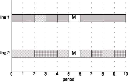
and resulted in the optimal solution listed in figure 2, with objective function value of 277,620
dollars. Figure 3 shows the inventories and backorders of the optimal solution.

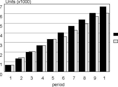
Cumulative capacity

Cumulative demand

Figure 1: Cumulative demand versus cumulative capacity

□product 1

□product 2

□product 3

□product 4

□product 5
∣M] maintenance

□idletime

Figure 2: Optimal schedule for basic scenario

The three other scenarios referred to earlier, are summarized table 6.

In the first scenario, the setup costs of product 1 were increased to 3,000 dollars. As expected, the
original optimal solution remained unchanged, because the increase in setup costs does not
exceed the backorder costs of products 2 and 3 that would be rescheduled to save one setup of
product 1. These results further validate our model.

The second scenario reduces the capacity of the second (cheaper) production line by 50%,
resulting in a drastic increase in the number of backorders. Again, this result is to be expected,
and is listed in table 7. Note that the model chose to give priority to the product with the highest
total demand. The objective function value rose to 443,960 dollars. The third scenario then
consisted of increasing the backorder costs of product 1. One would expect that in this case the
model would try to avoid shortages of this product, which resulted. The total costs amounted to
334,270 dollars.

<<   8   9   10   11   12   13   14   >>

More intriguing information