The name is absent

Simplifying, in the special case that v = O, equations (11) and (26) collapse to

^t + — (yt — yt_i ) = ^{o,                                 (2}7⁾

к

πt + ^—yt = O,                              (28)

к

respectively. It follows that the state is described by u_t for the discretionary policy, by u_t
and λ_πt for the optimal commitment policy, and by u_t and y_t_i for the timeless perspective
policy. As I now illustrate numerically,⁸ the performances associated with each of these
policies depends importantly on how these differences among the state variables is treated.

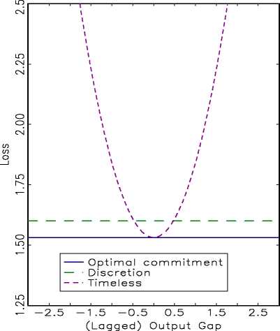
A: Conditional Loss

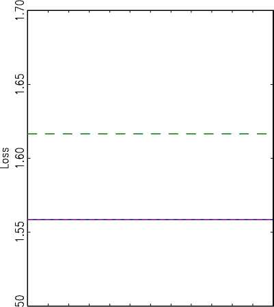
B: U n co nd ition a I Loss

—’ — 2.5 -1.5 -0.5  0.5   1.5   2.5

(Lagged) Output Gap

Fig. 1

One way to measure the performance of each policy is to simply evaluate equation (14)
conditional on the relevant initial states. For the optimal commitment policy and the dis-
cretionary policy, it is straightforward to evaluate equation (14), since both policies assume
a given known value for uŋ and since for the optimal commitment policy it is known that
Λ_πo = O. It is slightly more complicated for the timeless perspective policy, since that policy
requires an initial value for y_i, the lagged output gap.

Consider Figure 1A, which displays performances for uo = O and for an array of different
initial values for the lagged output gap. By construction, the optimal commitment policy
⁸I parameterize the model according to к = 0.025, ρ_u = 0.20, β = 0.99, σ_eu = 1, and μ = 0.50.

11

<<   10   11   12   13   14   15   16   >>

More intriguing information