Non-causality in Bivariate Binary Panel Data

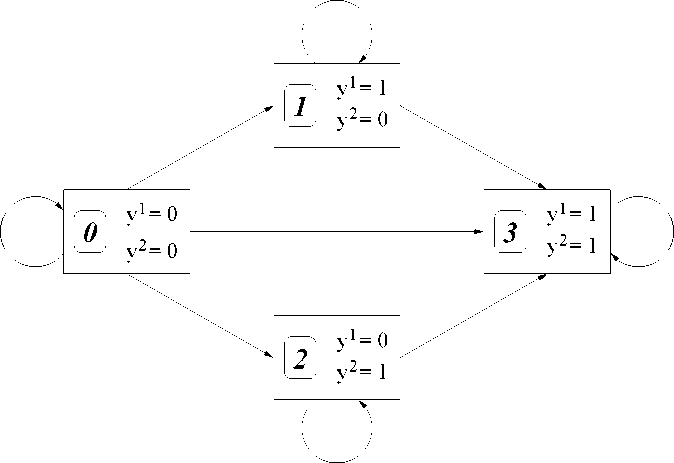
Figure 2: State-Transition Diagram for a Bivariate Survival Model

Conditions for simultaneous independence and Granger поп-causality can be
easily adapted from those introduced in Section 2, and take the particularly
simple form:

Also the introduction of exogenous variables can be accounted for by simply
paralleling the solutions presented in Section 3. The same holds true as regards
the introduction of the lagged dependent variables yi,t-j', saturated and unsat-
urated models are defined as in Section 3, but a comment is in order: in this
case conditioning on the lagged endogenous variables is meaningful only when
the individual is in state 1 or 2, since when he is in state 0, conditioning on this
information induces no change in the transition probabilities, as state 0 cannot
be accessed from any other state of the model.

As for the asymptotic properties of the estimates and tests, notice that for
this model, even in the case of homogeneous populations, Proposition 5 does not
hold, since this model can be represented as a Markov chain with an absorbing
state corresponding to state 3. This means that N —> ∞ is needed in order
to ensure consistency and asymptotic normality of the estimates. Conversely,
T —> ∞ does not lead to the usual asymptotic properties. The intuition is that,
for any finite N, when T —> ∞ all individuals will eventually end up in the

16

<<   13   14   15   16   17   18   19   >>

More intriguing information