averse or because he faces higher variance in his income. Hence, these latter two
parameters can be jointly identified, ρσs2 , as both act on the producer’s risk premium in
a similar way.
For the purposes of the simulation, we consider an identical number of processors
and growers, varying from 1 to 40, in steps of 5. Likewise, we assume that ρσs2 to take
values 0, 0.000001, 0.00001 and 0.00018. Still larger values for ρσs2 do not
substantially affect the results of simulation exercise reported in this section. Using the
equations explained in the models, we calculate the grower’s effort in quantity in each
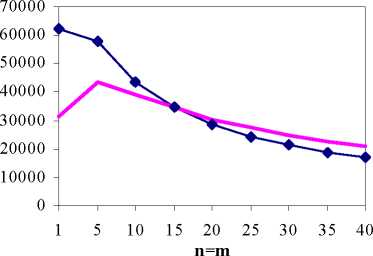
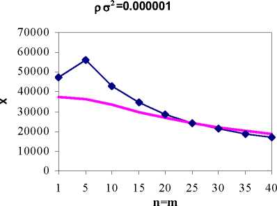
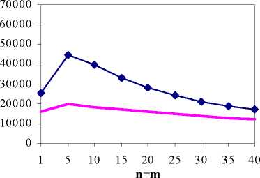
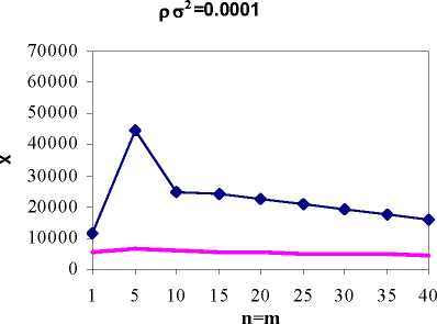
contractual mechanism for each of possible combinations, which is illustrated in Figure
1. This process has been repeated for the grower’s effort in quality and the total certain
equivalent (see figures 2 and 3, respectively).
ρσ2=0


ρ σ2 =0.00001


♦----♦ Incentive Contract Market
Figure 1. Comparing grower’s effort in quantity with incentive contract and spot market
More intriguing information
1. The name is absent2. Beyond Networks? A brief response to ‘Which networks matter in education governance?’
3. The name is absent
4. Nach der Einführung von Arbeitslosengeld II: deutlich mehr Verlierer als Gewinner unter den Hilfeempfängern
5. Cyclical Changes in Short-Run Earnings Mobility in Canada, 1982-1996
6. The Response of Ethiopian Grain Markets to Liberalization
7. Legal Minimum Wages and the Wages of Formal and Informal Sector Workers in Costa Rica
8. Cultural Diversity and Human Rights: a propos of a minority educational reform
9. Proceedings from the ECFIN Workshop "The budgetary implications of structural reforms" - Brussels, 2 December 2005
10. The name is absent