Accurate and robust image superresolution by neural processing of local image representations

In table 1 are presented the root mean squared (RMS) errors for different irregular
interpolation methods. Polynomial models with orders ranging from 1 to 3 have been
considered. For comparison, the error corresponding to the direct selection of the
nearest pixel (SEQ_NN) has been included, together with two distance-based interpo-
lators: the first processing step of our previous method (MLP-PNN), and a method re-
cently proposed in the literature [10], which makes use of inverse distance weights.
As it can be observed, interpolation with second order local polynomials provides dis-
tinct advantages over distance-based methods at low and medium noise levels. In-
creasing polynomial order over this point result only in marginal gains in perform-
ance. In view of these results, a second order polynomial has been considered in our
subsequent work.

Dimensionality reduction by PCA. Eigenimages of coefficients

The dimension of network input space is given by the model dimension (6 for a sec-
ond order polynomial) times the size of the considered local neighborhood. Principal
component analysis (PCA) has been applied to reduce the dimensionality of this
space. PCA [11] is a linear technique that yields minimal representational error (in
terms of mean squared error, MSE) for a given reduction in the dimensionality space.
PCA operates by projecting the input data onto an orthogonal basis of the desired di-
mension, where the basis vectors are the eigenvectors of the input data covariance
matrix, ranked in order of decreasing eigenvalues.

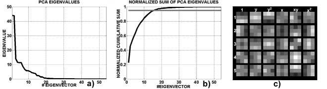
Fig. 1. Results of the PCA process, for a 3x3 local neighborhood: a) eigenvalues sorted in de-
creasing order; b) percentage of input variance maintained after dimensionality reduction, as a
function of the number of used eigenvectors; c) first five eigenimages.

In figure 1 a, b) are presented, for a 3x3 local neighborhood, the obtained eigen-
values sorted in decreasing order, and the percentage of the input variance represented
after dimensionality reduction, as a function of the number of used eigenvectors. Us-
ing a common heuristic approach, such as maintaining enough components to explain
95% of the input variance, will lead to the selection of the first 16 eigenvectors to
build the projection basis. In the next section we will see that heuristics of this type
are not appropriate for this problem, as use of low variance eigenvectors can have a
considerable impact on the final prediction error.

In figure 1 c) are presented the five eigenvectors of highest eigenvalue, with com-
ponents rearranged in the form of eigenimages. The preliminary experiments con-
ducted show their stability under variations of input noise and image content, defining
basic patterns of spatial variation of local polynomial models in images examined at

<<   1   2   3   4   5   6   >>

More intriguing information