Journal of Vision (2007) 7(8):1, 1-12
Schofield, Ledgeway, & Hutchinson
patterns, we spatially shifted each horizontal row of pixels
in the noise carrier image in the horizontal dimension by
an amount and direction (either leftward or rightward) that
was determined by the drifting sinusoidal waveform. This
resulted in a motion sequence in which the local
orientation of the striped elements within the dynamic
noise was modulated over space and time.
The modulation depth of all signals could be varied
within the range 0 to 1 according to the following
equations. The LM modulation depth (ML) was given by
ML = (Lmax j Lmin)/(Lmax + Lmin), where Lmax and Lmin
refer to the maximum and the minimum luminances,
respectively, averaged over adjacent noise stripes with
opposite polarity in the image. For CM, MC = (Cmax j
Cmin)/(Cmax + Cmin), where Cmax and Cmin refer to the
maximum and the minimum local Michelson contrasts,
respectively, in the image computed over adjacent noise
stripes with opposite polarity. For OM, MO = (Omax j
Omin)/90, where Omax and Omin refer to the maximum and
the minimum local orientations, respectively, in the image
computed relative to a reference orientation of 90-
(corresponding to vertical).
The total stimulus duration was 1 s, although the on and
off transitions were smooth with a raised cosine profile
lasting 200 ms. Similarly, stimuli were spatially win-
dowed in the vertical dimension according to a half cycle
of a raised cosine function with a half period of 1 deg
(not shown in the movies). These manipulations mini-
mized the presence of spatial and temporal transients.
Procedure and analysis
Modulation thresholds for discriminating the direction
of motion were measured over a range of spatial (Experi-
ment 1) and temporal (Experiment 2) frequencies. Motion
stimuli were presented in a single-interval, two-alternative
forced-choice design where the observer had to indicate
the direction of motion (up vs. down) using one of two
response buttons. Stimulus modulation depth on each trial
was chosen at random from a set of nine predetermined
values, selected based on pilot studies. In Experiment 1,
data were collected for spatial frequencies in the range
0.125-4 c/deg (maximum of 2 c/deg for P.D.J.) at a fixed
temporal frequency of 1 Hz. In Experiment 2, data were
collected for temporal frequencies in the range 0.5-9.5 Hz
at a fixed spatial frequency of 0.5 c/deg. Conditions were
blocked such that only one cue type and frequency were
tested in a given session. Observers completed four
sessions of 70 trials for each spatial and temporal
frequency tested. Data were fitted with Weibull (1951)
functions from which 75% correct thresholds were
extracted. Sensitivity was calculated as the reciprocal of
the threshold modulation depth.
Results
Experiment 1
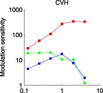
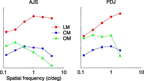
Sensitivity curves for direction discrimination versus
spatial frequency are plotted in Figure 1. Sensitivity for
LM appears high pass because we did not test at high
enough spatial frequencies to obtain the expected band-
pass response. Sensitivity for LM was maximal at about
1-2 c/deg. Sensitivity for CM was band pass with a peak
at 1 c/deg, but unlike LM, sensitivity reduced rapidly with
further increases in frequency. Sensitivity for CM was
considerably lower than that for LM across the range.
Sensitivity for OM was more low pass than for CM with a
knee between 0.5 and 1 c/deg (except for A.J.S.) with an
acute reduction in sensitivity beyond the knee. These results
are consistent with previous findings suggesting that
sensitivity for second-order cues is much lower than that
for first-order cues but that sensitivity curves for CM and LM
have broadly similar shapes whereas those for some other
types of second-order cue are more low pass (Hutchinson &
Ledgeway, 2006; Lu & Sperling, 2001). However, we note
that first-order sensitivity can depend on the type of
noise used (Lu & Sperling, 2001; Schofield & Georgeson,


Figure 1. Sensitivity as a function of spatial frequency; circles, squares, and triangles show sensitivity to LM, CM, and OM, respectively.
Error bars show 95% confidence intervals estimated from 5,000 iterations of a nonparametric bootstrap procedure.
More intriguing information
1. Structural Breakpoints in Volatility in International Markets2. The name is absent
3. Literary criticism as such can perhaps be called the art of rereading.
4. A Rare Case Of Fallopian Tube Cancer
5. The Dynamic Cost of the Draft
6. Response speeds of direct and securitized real estate to shocks in the fundamentals
7. The name is absent
8. Økonomisk teorihistorie - Overflødig information eller brugbar ballast?
9. FUTURE TRADE RESEARCH AREAS THAT MATTER TO DEVELOPING COUNTRY POLICYMAKERS
10. The name is absent