18
where the time constants are
T^L = Cτn∕∂Li ^^Na — Cm∣ C)Na, and 7⅛ — Cm∕ Qκ∙
Representing the quasi-active system as a linear system permits both an analytic solu-
tion via the eigenvalue decomposition and also a description of the resonant behavior
of (2.3) in terms of the eigenvalues of A.
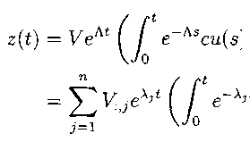
Recall that the linear system given in (2.12) has the analytic solution
z{t) = eAt ( [ e~AsBu(s)ds + z(0)^ . (2∙14)
Vo /
Assuming A is diagonalizable, it has an eigenvalue decomposition
A = RAIZ-1, (2.15)
where A is a diagonal matrix. That is, the jth column of V is the eigenvector corre-
|
Sponding to the eigenvalue A7 = z(t) = VeAt n =Σ'∙ J=I |
= Λj∙j∙. Then substituting (2.15) into (2.14) yields ( /" e~Ascu(s)ds + z(0)^ Vo / r∙je^t f [ e~λjsCju(s)ds + ¾(0)λj , |
where c = V λB, which is a vector in this example system. The integral can be
More intriguing information
1. Altruism with Social Roots: An Emerging Literature2. Spatial Aggregation and Weather Risk Management
3. National curriculum assessment: how to make it better
4. A Dynamic Model of Conflict and Cooperation
5. Pass-through of external shocks along the pricing chain: A panel estimation approach for the euro area
6. Human Rights Violations by the Executive: Complicity of the Judiciary in Cameroon?
7. Epistemology and conceptual resources for the development of learning technologies
8. Fiscal Insurance and Debt Management in OECD Economies
9. Quality Enhancement for E-Learning Courses: The Role of Student Feedback
10. The name is absent