The name is absent

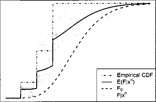
Figure 3.1: Base measure Fo=Gα(9,2), posterior base measure Fi := F(F ∣ τⁿ), empirical
cdf and set of simulated measures sampled from the posterior distribution of the DP (a =
5, Fo) when a sample xⁿ: 1,2,2,3,3 and 3 of this DP was observed.

3.1 shows the base measure Fq=G<z(9,2), the posterior base measure F₁, the empirical
cdf and a set of simulated measures sampled from the posterior distribution of the
DP(θ! = 5, F₀) via (3.5) when the sample of size n = 6 of this DP: 1,2,2,3,3 and 3
was observed.

The DP allows analytic evaluation of the marginal distribution p(X₁,... ,X_n),
integrating with respect to F ~ DP(a, F₀). The marginal distribution is also known
as the Polya urn (Blackwell and MacQueen₁ 1973). We will exploit the Polya urn later
in this section to simulate from a DP. This representation, in particular, implies that
if Xι,... ,X_n is a random sample of this sample: X₁,... ,X^ are a random sample
from Fq. This implies that

Pr[Xι ∈ ∙] = F_o(∙).

<<   53   54   55   56   57   58   59   >>

More intriguing information