Determinants of Household Health Expenditure: Case of Urban Orissa

COEFFICIENTS

a Dependent Variable: PHE

Source: Compiled from Primary Data

From the study it is found that as disposable
income (Yd) of the household increases,
individual takes more care of his life, hence
health expenditure (H) increases but at a
particular level of income, due to high life
risk, health expenditure becomes
independent of income and perfectly elastic,
which is termed as “High Life Risk Path
(HLRP)”. The health expenditure during
HLRP depends on household’s past saving
(S) and loanable capacity (L).

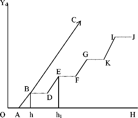
FIGURE 2

THE HEALTH EXPENDITURE CURVE

In figure 2, OA is autonomous health expenditure. In normal life, ABC is the health

expenditure curve (with linear relationship assumption between health expenditure and
disposable income) without any high life risk. But due to high life risk at Bh level of disposable
income, B is the bearable point³ and BD is the HLRP. Again normal life starts from point D to
point E. At Eh1 level of disposable income, E is the bearable point and EF is the HLRP and so
on. Hence, ABDEFGKIJ is the health expenditure path at high life risk, which is not a normal
path.

³ The bearable point is the point at which the maximum health expenditure can be financed from a particular level of
disposable income.

<<   3   4   5   6   7   8   >>

More intriguing information