Business Cycle Dynamics of a New Keynesian Overlapping Generations Model with Progressive Income Taxation

4.2 Productivity shock

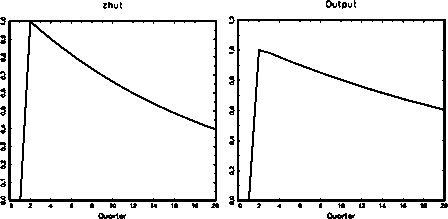
In Figure 2, the impulse response functions of aggregate variables to a technology shock
εz,2 = 1 in period 2 (and zero thereafter) are presented. In the first row, the percent-
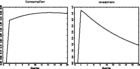
age deviations of the variables technology level zt , output Yt , consumption Ct , and
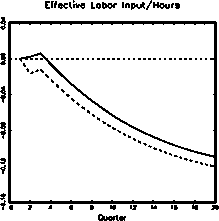
investment I_t are graphed, in the second row, we illustrate the percentage deviations
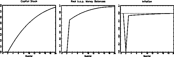
of effective labor input N_t and working hours (the dotted line), capital K_t, real money
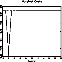
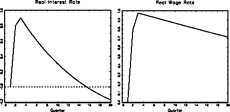
mt , and the inflation factor πt , while in the third row, you find the behavior of marginal
costs g_t (the inverse of the mark-up), profits Ω_t, the real interest r_t, and the wage rate

^wt^.

Figure 2

Technology Shock in the OLG Model

Following an unexpected increase of the technology level by 1%, output increases by
1.0% as well. On impact, effective labor input increases slightly whereas working hours
decrease. Subsequently both effective labor input and hours decrease. This result stems

17

<<   16   17   18   19   20   21   22   >>

More intriguing information