Macroeconomic Interdependence in a Two-Country DSGE Model under Diverging Interest-Rate Rules

7. Impulse-Response Analysis

impulses in period 1 on the exogenous error terms η_a, η*, η_u, ηU, η_v ,ηV in terms of one standard deviation
of +л/0Л on their expected value of 0. The impulse-response analysis is carried out by employing the
Dynare package for Matlab while simulating over 2100 periods.²⁸ For the Dynare program code see
Appendix A.6.

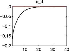
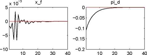
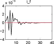
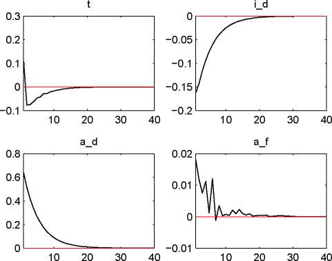
The six figures below show the responses of the output gaps x, x*, PPI inflation rates πH, ∏F, movements
in the TOT ∆t, nominal interest rates i, i*, and the relevant shock variables themselves to (orthogonalized)
impulses on the various exogenous error terms for a time range of 40 periods or 10 years.²⁹

x 10—4      Pi^_f

151-----■------—

-51------------■-------------■-------------■-------------

10   20   30   40

Figure 1: Responses to an impulse on the domestic productivity shock

²⁸The software is downloadable from http://www.cepremap.cnrs.fr/dynare/. For all computations associated with the
impulse-response analysis it uses the pure perturbation algorithm developed by Schmitt-Grohe/Uribe (2004, pp.
764-765) as its default option.

²⁹Note that the following is assumed for the variance-covariance matrix of the various exogenous error terms:

22

<<   20   21   22   23   24   25   26   >>

More intriguing information