Geography, Health, and Demo-Economic Development

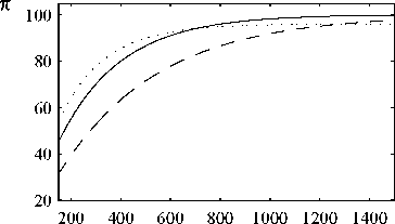
86 countries). One sees that the endogenously generated child survival function approximates
the estimate quite well.

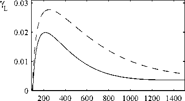
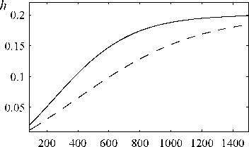
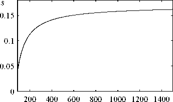
Figure 4: Correlations of Demo-Economic Development

βι = 0.32, β2 = 0.09, вз = 0.12, β4 = 0.87, λ = 5, с = 67, a = 0.72, and b = 0.004 (solid lines) and
0.0025 (dashed lines). Dotted line: estimate of the child survival function in Kalemli-Ozcan (2002,
Table 3).

Dashed lines in Figure 4 show behavior of families living in an unfavorable environment (e.g. a
tropical region) where fundamental child survival improves less quickly when income per capita
rises. For that purpose we set b = 0.0025 and keep everything else from the U.S. calibration.
Population growth peaks now at a higher level and decays less quickly. At the peak a couple of
adults gives birth to 5 children generating a population growth rate of 2.8 percent. These values
correspond approximately with the facts observed for the poorest countries in Sub Saharan
Africa.

The model suggests that the income correlations in Figure 1 will be observed along a path
of successful demo-economic development. That households generate these correlations does,
however, not imply that successful development will actually happen. To answer the questions
of if and when a demographic transition occurs and how long it will then take to arrive at the
stage of a fully developed economy we place households in a macro-economy and investigate the
dynamic consequences of their actions.

13

<<   12   13   14   15   16   17   18   >>

More intriguing information