20
1 Stable distributions
Stable and Gaussian fit to Boeing returns

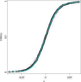
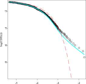
Figure 1.7: Stable (cyan) and Gaussian (dashed red) fits to the Boeing stock
returns (black circles) empirical cdf from the period July 1, 1997 -
December 31, 2003. Right panel is a magnification of the left tail
fit on a double logarithmic scale clearly showing the superiority of
the 1.78-stable law.
θ STFstab07.xpl
Stable, Gaussian, and empirical left tails

log(x)
us to accept the α-stable law as a model of DJIA returns. The values of the
test statistics for the Gaussian fit yield p-values of less than 0.005 forcing us to
reject the Gaussian law, see Table 1.1.
Next, we apply the same technique to 1635 daily returns of Boeing stock prices
from the period July 1, 1997 - December 31, 2003. The 1.78-stable distribution
fits the data very well, yielding small values of the Anderson-Darling (0.3756)
and Kolmogorov (0.4522) test statistics, see Figure 1.7 and Table 1.2. The
approximate p-values based, as in the previous example, on 1000 simulated
samples are 0.18 and 0.8, respectively, allowing us to accept the α-stable law as
a model of Boeing returns. On the other hand, the values of the test statistics
for the Gaussian fit yield p-values of less than 0.005 forcing us to reject the
Gaussian distribution.
The stable law seems to be tailor-cut for the DJIA index and Boeing stock
price returns. But does it fit other asset returns as well? Unfortunately, not.
Although, for most asset returns it does provide a better fit than the Gaussian
More intriguing information
1. The name is absent2. Computational Experiments with the Fuzzy Love and Romance
3. Developments and Development Directions of Electronic Trade Platforms in US and European Agri-Food Markets: Impact on Sector Organization
4. AN IMPROVED 2D OPTICAL FLOW SENSOR FOR MOTION SEGMENTATION
5. The name is absent
6. STIMULATING COOPERATION AMONG FARMERS IN A POST-SOCIALIST ECONOMY: LESSONS FROM A PUBLIC-PRIVATE MARKETING PARTNERSHIP IN POLAND
7. FOREIGN AGRICULTURAL SERVICE PROGRAMS AND FOREIGN RELATIONS
8. Computing optimal sampling designs for two-stage studies
9. WP 1 - The first part-time economy in the world. Does it work?
10. The name is absent