Stable Distributions

1.6 Financial applications of stable laws

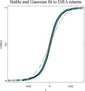
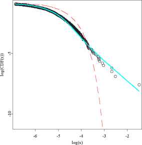
Figure 1.6: Stable (cyan) and Gaussian (dashed red) fits to the DJIA returns
(black circles) empirical cdf from the period February 2, 1987 -
December 29, 1994. Right panel is a magnification of the left tail
fit on a double logarithmic scale clearly showing the superiority of
the 1.64-stable law.

θ STFstab06.xpl

Stable, Gaussian, and empirical left tails

puts more weight to the differences in the tails of the distributions. Although
no asymptotic results are known for the stable laws, approximate p-values for
these goodness-of-fit tests can be obtained via the Monte Carlo technique.
First the parameter vector is estimated for a given sample of size n, yielding
θ, and the test statistics is calculated assuming that the sample is distributed
according to F (x; θ), returning a value of d. Next, a sample of size n of F (x; θ)-
distributed variates is generated. The parameter vector is estimated for this
simulated sample, yielding θ1, and the test statistics is calculated assuming that
the sample is distributed according to F (x; θ1). The simulation is repeated as
many times as required to achieve a certain level of accuracy. The estimate of
the p-value is obtained as the proportion of times that the test quantity is at
least as large as d.

For the α-stable fit of the DJIA returns the values of the Anderson-Darling and
Kolmogorov statistics are 0.6441 and 0.5583, respectively. The corresponding
approximate p-values based on 1000 simulated samples are 0.02 and 0.5 allowing

<<   17   18   19   20   21   22   23   >>

More intriguing information