Stable Distributions

1 Stable distributions

S0 parameterization

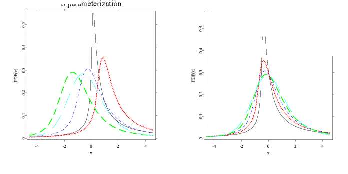
S parameterization

Figure 1.3: Comparison of S and S⁰ parameterizations: α-stable pdfs for β =

0.5 and α = 0.5 (black solid line), 0.75 (red dotted line), 1 (blue
short-dashed line), 1.25 (green dashed line) and 1.5 (cyan long-
dashed line).

θ STFstab03.xpl

1.3.2 Stable density and distribution functions

The lack of closed form formulas for most stable densities and distribution
functions has negative consequences. For example, during maximum likeli-
hood estimation computationally burdensome numerical approximations have
to be used. There generally are two approaches to this problem. Either the
fast Fourier transform (FFT) has to be applied to the characteristic function
(Mittnik, Doganoglu, and Chenyao, 1999) or direct numerical integration has
to be utilized (Nolan, 1997, 1999).

For data points falling between the equally spaced FFT grid nodes an inter-
polation technique has to be used. Taking a larger number of grid points in-
creases accuracy, however, at the expense of higher computational burden. The
FFT based approach is faster for large samples, whereas the direct integration
method favors small data sets since it can be computed at any arbitrarily cho-
sen point. Mittnik, Doganoglu, and Chenyao (1999) report that for N = 2¹³
the FFT based method is faster for samples exceeding 100 observations and

<<   4   5   6   7   8   9   10   >>

More intriguing information