Manufacturing Earnings and Cycles: New Evidence

plained and an unexplained part,

= ^sc(^ω)fy(^ω) + ∕4^ω)∙

Integrating equation (4) over the frequency band [—7r,7r] gives

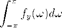
^⅛(o)

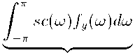
“explained” variance

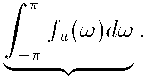
σ²

The first term on the right in equation (4') is the product of squared coherency
between X_t and Y_t and the spectrum of Y_t∙, the second term is white noise. This
equality holds for every frequency band [ωι,ω₂]. We can plot total variance
(the area under the spectrum) and explained variance as shown in Figure 2.
Comparing the area under the spectrum of the explained component to the
area under K’s spectrum in a frequency interval [ω₁,ω₂] yields a measure of the
explanatory power of X, analogous to an R² in the time domain. In contrast
to sc however, R² is constant across all frequencies.

spectrum is the Fourier transform of the cross-covariance function:

₁ ∞

fyA^ω) = χ- ∑2 7^(C^e^^ωτ; ^ω ∈ [-fo4
Z7Γ '

T = -OO

<<   5   6   7   8   9   10   11   >>

More intriguing information