Stakeholder Activism, Managerial Entrenchment, and the Congruence of Interests between Shareholders and Stakeholders

welfare.

Example 1 In figure 3 we set θ_I = .1, θ_R = .5, α = .5, p = .5, τ = .5, λ = .7, a = .4, B = 2
and Γ = 0.8. With these parameters π* = 0.44 and b_r(π*) = 0.47 .

Example 2 In figure 4 we keep the same data of example 1 but assume that both the
stakeholder ability at affecting the replacement decision, and the incumbent control benefits
are higher (i.e. we set a = .8 and Γ = 2). In this case: π* = 0.038 and b_r(π*) = 0.063.

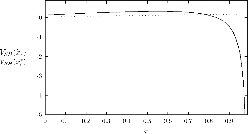
Figure 3: The continuous (dotted) curve represents shareholder value when entrenchment is
(not) to be countered. Shareholders preempt entrenchment: π^* = 0.44 and xb_r(π^*) = 0.47.

Notice that in both examples shareholder value is indeed maximized by countering man-
agerial entrenchment (i.e., it is not optimal to set π and xr below the xbr(π) locus). Therefore,
we can conclude:

Proposition 2 There is an open set of parameters for which shareholder value is maximized
by countering managerial entrenchment, and hence by providing a minimal level of explicit
stakeholder protection xbr (π^*) > 0.

Remark 2 — Welfare effects — To be written.

17

<<   14   15   16   17   18   19   20   >>

More intriguing information