Stata Technical Bulletin
23
the value of the Jth В-spline at the ith reference point. If β is the (column) '/-vector of regression coefficients with respect to
the В-splines in V, and 7 is the (column) <∕-vector of values of the spline at the reference points, then
7 = Wβ (7)
If W is invertible, then the «-vector of values of the fitted spline at the data points is
V β = VW~1Wβ = UIΓlo = Z7 (8)
where Z = VW 1 is a transformed n × d design matrix whose columns contain values of a set of reference splines for the
estimation of the reference-point spline values 7.
The choice of reference points is open to the user and constrained mainly by the requirement that the matrix W is invertible.
This implies that each of the q В-splines must be positive for at least one of the q reference values, and that each reference
value must have at least one positive В-spline value. A natural choice of reference values might be one in the midrange of each
В-spline, possibly the central knot for an odd-degree В-spline (such as a linear, cubic, or quintic), or the midpoint between the
two central knots for an even-degree В-spline (such as a constant, quadratic, or quartic). This choice has the consequence that,
for a spline of degree kt there will be int(⅛∕2) reference points outside the spline’s completeness region on the left, and another
int(⅛∕2) reference points outside the spline’s completeness region on the right. The parameters corresponding to these “extra”
reference points will not be easy to explain to nonmathematicians, as they describe the behavior of the spline as it returns to
zero outside its completeness region. However, for a quadratic or cubic spline, there is only one such external reference Y -value
at each end of the range.
By default (if the user does not specify knots), frencurv starts with the reference points originally provided (which default
to the minimum and maximum of xvar if no ref pts are provided) and chooses knots “appropriately.” For an odd-degree spline
(power odd), the knots are initialized to the original reference points themselves. For an even-degree spline (power even), the
knots are initialized to midpoints corresponding to the original reference points. That is to say, if there are m original reference
points r± < ... < rm and power is even, then the original knots s0 < ... < sto are initialized to
f ri - (r2 -rι)∕2, if j = O
Sj = < f +rj∙+ι)∕2, ifl≤J≤m-l (9)
[ fto + irm - fto-i)∕2, if j = m
frencurv assumes, by default, that the reference points initially provided are all in the completeness region. It adds
int(⅛∕2) extra reference points to the left, spaced by the difference between the first two original reference points, and int(⅛∕2)
extra reference points to the right, spaced by the difference between the last two original reference points, where к is specified
by the power option. If noexref is specified, then the original refpts are assumed to be the complete set, and it is the user’s
responsibility to choose sensible ones. In either case, the original knots are extended on the left and right as described above,
unless noexknot is specified. (These rules seem complicated, but lead to sensible defaults if the naive user specifies a list of
reference points and expects them to be in the completeness region of the spline, while preserving the ability of advanced users
to specify exactly what they want at their own risk.)
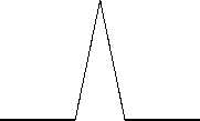
Figure 2 shows the constant, linear, quadratic and cubic reference splines corresponding to a reference point at 4, assuming
unit reference points and default knots (equal to reference points for odd degree and inter-reference midpoints for even degree).
Note that each spline is one at its own reference point and zero at all other reference points. They are similar to (but not the
same as) the В-spline wavelets of Unser et al. 1992.
1.00 ∙
0.75 ∙
0.50 ∙
0.25 ∙
0.00 ∙

1.00
0.75
0.50
0.25
0.00
— 0.25 ^* . . . . . . . . . —0.25 ^∣
012345678 012345678

More intriguing information
1. The technological mediation of mathematics and its learning2. The name is absent
3. Spatial Aggregation and Weather Risk Management
4. Publication of Foreign Exchange Statistics by the Central Bank of Chile
5. Multifunctionality of Agriculture: An Inquiry Into the Complementarity Between Landscape Preservation and Food Security
6. Improvement of Access to Data Sets from the Official Statistics
7. Barriers and Limitations in the Development of Industrial Innovation in the Region
8. Economie de l’entrepreneur faits et théories (The economics of entrepreneur facts and theories)
9. TLRP: academic challenges for moral purposes
10. Growth and Technological Leadership in US Industries: A Spatial Econometric Analysis at the State Level, 1963-1997