The name is absent

Figure 2. Reference splines at 4 with unit reference points.

Example

In Stata’s auto data, we can use frencurv and regress (with the noconstant option) to fit a cubic spline for miles per
gallon with respect to weight:

. frencurv,xvar(weight) refpts(1760(770)4840) gen(cs) power(3)

. describe cs*

We have arbitrarily chosen the reference points to be equally spaced from the minimum of weight (1,760 pounds) to
the maximum of weight (4,840 pounds). By default, frencurv ensures that the spline is complete in the range of X-values
spanned by the original reference points provided by the user. The describe command lists the reference splines with their
labels. Note that frencurv has added two extra reference points outside the spline’s completeness region (at weights of 990 and
5,610 pounds) and indicated this incompleteness in the variable labels. The coefficients fitted by regress (with the noconstant
option) are simply the fitted values of mpg at the reference points. Note that the ones corresponding to the splines cs2 to
cs6 have “sensible” values, corresponding to the expected levels of mpg at the appropriate value of weight, whereas the ones
corresponding to csl and cs7 have “nonsense” values because they correspond to reference “weights” extrapolated off the edge
of the range of sensible weight values. This is the price we pay for making all reference points equal to knots of the cubic
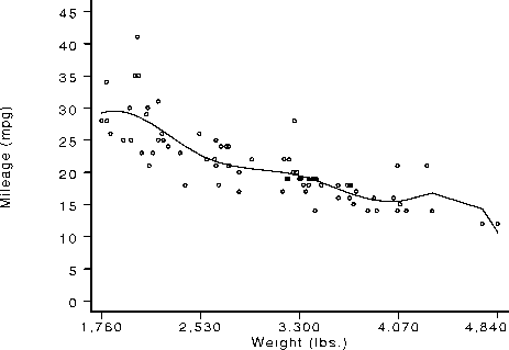
spline. Figure 3 shows observed and fitted values of mpg plotted against weight. The fitted curve is calculated using predict
(see [R] predict) and is interpolated cubically between the reference points.

Figure 3. Mileage plotted against weight (points) with fitted cubic spline (line).

The f rencurv parameterization allows us to use Iincom to calculate confidence intervals for differences (or other contrasts)

<<   21   22   23   24   25   26   27   >>

More intriguing information