22
Stata Technical Bulletin
STB-57
The scaled В-spline A(χ∙, sɪ,..., sa+t) has the advantage that it is dimensionless, being a sum of products of the dimensionless
quantities φhj{x). That is to say, it is unaffected by the scale of units of the ж-axis, and therefore has the same values, whether
ж is time in millennia or time in nanoseconds. The original Ziegler В-spline В(ж; sɪ,..., s∕e+2) is expressed in units of ж-1.
Therefore, if the scaled В-spline А(ж;sɪ,... ,Sfe+2) appears in a design matrix, then its regression coefficient is expressed
in units of the У-variate, whereas if the original В-spline В(ж; sɪ,..., s∕e+2) appears in a design matrix, then its regression
coefficient is expressed in Y-units multiplied by X-units and will be difficult to interpret, even for a mathematician. The B-splines
computed by bspline are therefore the А(ж; sɪ,..., ⅝+2), and users who prefer the original Ziegler В-splines must scale
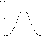
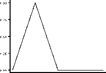
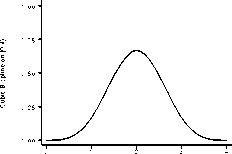
them by (⅛ + l)∕(s⅛+2 — sɪ). (This factor happens to be one for splines with unit-spaced knots, such as those in Figure 1.)
0.00 ^* . . . ~
0 12 3


Figure 1. В-splines originating at zero with unit knots.
Givenndatapoints, a У-variate, an X-covariate, and a set of q + k+'∖ consecutive knots s⅛ < ...< s⅛+g < ... < s⅛+q+⅛,,
we can regress the У-variate with respect to a fcth-degree spline in X by defining a design matrix V, with one row for each of
the n data points and one column for each of the first q knots, such that
Vij = A(a⅛; s⅛ψj-ι, ∙ ∙ ∙, s⅛+j+fe) (5)
We can then regress the У-variate with respect to the design matrix V and compute a vector β of regression coefficients, such
that Vβ is the fitted spline. The parameter βj measures the contribution to the fitted spline of the В-spline originating at the
knot s⅛+j-ι and terminating at the knot s⅛+j∙+⅛. There will be no stability problems such as we are likely to have with the
original plus-function basis, as each В-spline is bounded and localized in its effect.
It is important to define enough knots. If the sequence of knots { *∙∕} extends to +∞ on the right and to —00 on the left,
then the fcth-degree В-splines A(∙; s⅛+j-ι,..., s⅛+j∙+⅛) on sets of к + 2 consecutive knots are a basis for the full space of
fcth-degree splines on the full set of knots. If S,(∙) is one of these splines, and [sj∙,sj∙+i) is an interval between consecutive
knots, then the values of В(ж) in the interval are affected by the к + 1 В-splines originating at the knots Sj-k, ...,Sj and
terminating at the knots Sj+±,... ,Sj+o+o. It follows that, if we start by specifying a sequence of knots s0 < ... < sto, and
we want to fit a spline for values of x in the interval [s0, sto), then we must also use к extra knots s-k < ... < s_i to the left
of s0 and к extra knots sm+1 < ... < sto+⅛ to the right of sm to define the m + к consecutive В-splines affecting S'(ж) for ж
in the interval [s0, sto). These m + k В-splines originate at the knots s-k,..., sto-i and terminate at the knots sɪ,..., sm+k,
respectively. Any spline S(∙), in the full space of fcth-degree splines defined using the full set of knots, is equal to a linear
combination of these m + k В-splines in the interval [s0, sto), which we will denote as the completeness region for splines
which are linear combinations of these m + k В-splines. These linear combinations are zero for ж < *•_/,. and ж ≥ am+k and
“incomplete” in the outer regions [s-⅛,s0) and [sm,sm+k), in which the spline is “returning to zero”.
bspline and frencurv assume, by default, that the knots option specified by the user is only intended to span the
completeness region, and that the specified knots correspond to the so,...,sm. By default, bspline and frencurv generate
к extra knots on the left, with spacing equal to the difference between the first two knots, and к extra knots on the right, with
spacing equal to the difference between the last two knots. If the user specifies the option noexknot, then bspline assumes
that the user has specified the full set of knots, corresponding to ..., sto+⅛ and does not generate any new knots. This
allows users to specify their own spacing for the outer knots if they wish but makes the specification of knots simpler in the
default case because users do not have to count the extra outer knots for themselves.
The В-spline regression parameters are expressed in units of the У-variable, but they are not easy to interpret. If we have
calculated the n × m matrix V of B-splines as in (5), and we also have a set of q reference Х-values r∖<r∙2<---<r.,, then
we might prefer to reparameterize the spline by its values at the Tj. To do this, we first calculate a q × q square matrix W,
defined such that
(6)
Wij — Afa; S⅛+j-1, ∙ ∙ ∙ , Shj-jj-β)
More intriguing information
1. Survey of Literature on Covered and Uncovered Interest Parities2. Review of “From Political Economy to Economics: Method, the Social and Historical Evolution of Economic Theory”
3. The name is absent
4. Human Development and Regional Disparities in Iran:A Policy Model
5. The name is absent
6. Portuguese Women in Science and Technology (S&T): Some Gender Features Behind MSc. and PhD. Achievement
7. Strategic monetary policy in a monetary union with non-atomistic wage setters
8. Social Irresponsibility in Management
9. STIMULATING COOPERATION AMONG FARMERS IN A POST-SOCIALIST ECONOMY: LESSONS FROM A PUBLIC-PRIVATE MARKETING PARTNERSHIP IN POLAND
10. The name is absent