The name is absent

Stata Technical Bulletin

Generalized Lorenz Curves

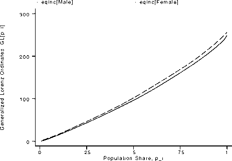
Figure 1. Generalized Lorenz curves for household incomes by head of household gender.

One may prefer to focus on comparisons of Lorenz curves for the two groups. In this case, we should first type the following
in order to construct the income measure divided by the relevant subgroup average:

. generate eqinc.m = eqinc

. for O l,l(n): su eqinc_-m if headfem==® // replace

> eqinc_m=eqinc_m/_result (3) if headfem==®

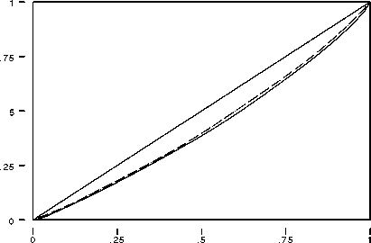
We can then build and draw the Lorenz curves, together with the 45 degree line which corresponds to the Lorenz curve
for a perfectly equal distribution, with the following commands:

. glcurve eqinc_-m, glvar(lc) pvar(p) by(headfem) split nograph

. graph lc_* p p ,s(...) c(lll) xlabel(0,0.25,0.50,0.75,1)

> ylab(0,0.25,0.50,0.75,1) yline(0_tl) xline(0_t 1) noaxis

eqinc_m[Male]
Cum. Pop. Prop.

eqinc_m[Female]

Population Share, p_i

Lorenz Curves

Figure 2. Comparing Lorenz curves for the two groups in Figure 1.

In order to illustrate the use of the sortvar(.) option, let us draw now a Concentration curve. Suppose we wish to see
how child benefits are distributed relative to the income distribution. Let us draw the Concentration curve of chpay (solid line)
along with the Lorenz curve of eqinc (dashed line).

. summarize eqinc

. replace eqinc_-m = eqinc∕_-result(3)

. glcurve eqinc_-m, gl(lc) p(p) replace nograph

. summarize chpay

. generate mchpay = chpay∕_-result(3)

. glcurve mchpay , gl(cc) sort(eqinc_-m) nograph

. graph Ic cc p p_t c(lll) s(...) xlabel(0,0.25,0.50,0.75,1)
> ylabel(0,0.25,0.50,0.75,1) yline(0_tl) xline(0_t 1) noaxis

<<   24   25   26   27   28   29   30   >>

More intriguing information