32
Stata Technical Bulletin
STB-58
(!weights or pweights) denoted by wŋ and cluster sequence numbers denoted by <¾. cendif follows the usual Stata practice
of assuming an fweight to stand for multiple observations with the same values for all other variables. The clusters may be
nested within the two groups or contain observations from each of the two groups, but the percentile differences will only apply
to observations from distinct clusters. If clusters are present, then the confidence intervals will be calculated assuming that the
sample was generated by sampling clusters independently from a population of clusters, rather than by sampling N observations
independently from the total population of observations or by sampling N1 and N2 observations from Populations A and B,
respectively. (By default, all the wŋ will be ones, and the <¾ will be in sequence from 1 to N. The difference between these
three alternatives will not matter.) We will denote by M the number of distinct values of a difference, Y1j — Y⅛⅛, observed
between Y values in the two samples belonging to different clusters. The difference values themselves will be denoted by
t1,... ,tjvf. For each ∕ι from 1 to M, we define the sum of product weights of differences equal to t⅛ as
Wh = δ{ci,ck}w1jw2k
(3)
j,k-.Ylj-Y2k=th
where δ(a,ty is 0 if a = a and 1 if a ≠ b. Given a value of θ expressed in units of Y, we can define Yζ(θ) to be Yij if i = 1
and Yij + θ if i = 2. The sample Somers’ D of Y*{θ) with respect to X is defined as
D*(ff) =P[Y*(0)∣X] =
∑J^ι ∑⅛fiι <K<¾, <⅞fe) w1jw2k sign(Yυ∙ - Y2k - θ)
∑^ι ∑k=ι S(clj,c2k) wljw2k
(4)
∑h∙.th>θ^ ∑h∙.th<e^h
Σ⅛
where D[∙ ∣ ∙] denotes the sample Somers’ D, defined by the methods of Newson (2000). Clearly, given a sample, D*(θ) is a
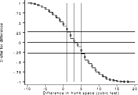
nonincreasing function of θ. (Note that only between-cluster differences are included.) Figure 1 shows D*(θ) as a function of
f for differences between trunk capacities of American and foreign cars (expressed in cubic feet) in the auto data. The squares
represent the values D*(t⅛) for the observed differences t⅛. Note that D*(θ) is discontinuous at the observed differences, and
constant in each open interval between two successive observed differences.

Figure 1. D* (O') plotted against the difference 0 in trunk space between American and foreign cars
We aim to include θ in a confidence interval for a gth percentile difference if, and only if, the sample D*(θ) is compatible
with a population Л[У* (0)∣X] equal to 1 — 2t∕. The methods of Newson (2000), used by the program somersd, typically
use a transformation ζ(∙), which, for present purposes, may either be the identity, the arcsine or Fishers’ z (the hyperbolic
arctangent). The transformed sample statistic ζ(θ) = ζ[D*(0)] is assumed to be normally distributed around the population
parameter ζ{D[y*(0)∣X]}. In the present application, we assume that if Л[У*(0)|У] = 1 — 2g, then the quantity
[¢(0) - ¢(1 - 2<z)] /SE[C(0)]
(5)
has a standard Normal distribution, where SE^(0)] is the sampling standard deviation (or standard error) of ^Z>*(0)]. If we
knew the value of SE^(0)], then a 100(1 — ct)% confidence interval for a gth percentile difference might be the interval of
values of θ for which
r1{ ¢(1 - 2<z) - za SE[f(0)] } ≤ D*(0) ≤ C1 { ¢(1 - 2<z) + za SE[f(0)] }
(6)
More intriguing information
1. The name is absent2. Political Rents, Promotion Incentives, and Support for a Non-Democratic Regime
3. Opciones de política económica en el Perú 2011-2015
4. On the Existence of the Moments of the Asymptotic Trace Statistic
5. On the Integration of Digital Technologies into Mathematics Classrooms
6. Regional specialisation in a transition country - Hungary
7. The name is absent
8. Deprivation Analysis in Declining Inner City Residential Areas: A Case Study From Izmir, Turkey.
9. Emissions Trading, Electricity Industry Restructuring and Investment in Pollution Abatement
10. Structural Conservation Practices in U.S. Corn Production: Evidence on Environmental Stewardship by Program Participants and Non-Participants