b

a
denotes the number of employees needed to serve 1000 customers in all services offering price
reductions in the interval [a,b] . In this case the ratio E/L is calculated according to the formula
(2.2)
R[d] = ∫ Φ [pr] ∫ Ψ[ "'] dwdpr
0 W[ pr,d]
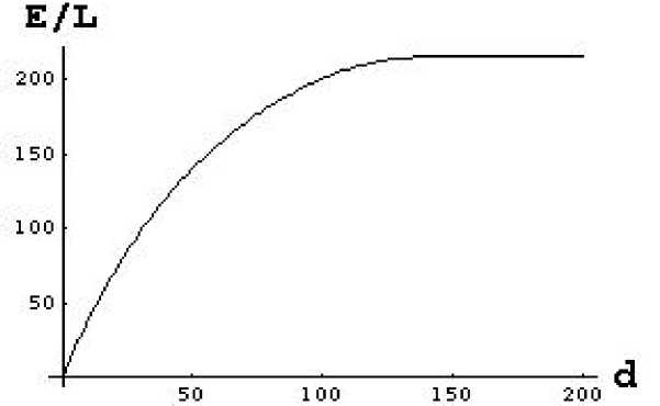
A numerical simulation making use of the result in (2.2) is shown in Figure 5.

Figure 5
Fractions of Employment/Labor as a
function of traveling distance d to CBD
The construction above ignores the
possibility of multipurpose shopping.
Conveniently rephrasing the problem,
however, we are able to include
multipurpose shopping within the
same setup. Consider the situation
shown in Table 1.
|
F1 |
F2 |
F3 | |
|
#Employees/1000customers |
10 |
30 |
20 |
|
Savings |
$10,00 |
$50,00 |
$60,00 |
|
Together with F1 only |
40 % |
10 % |
30 % |
|
Together with F2 only |
20 % |
60 % |
20 % |
|
Together with F3 only |
30 % |
10 % |
40 % |
|
F1, F2 and F3 |
10 % |
20 % |
10 % |
Table 1: Savings/shopping frequencies
As shown in Table 1, the customers will sometimes take advantage of more than one service at the
time. The idea is now simply to view a shopping combination as a new service. So we introduce new
combinations F4=(F1,F2), F5=(F1,F3), F6=(F2,F3) and F7=(F1,F2,F3). Using the conditional
frequencies from Table 1, we get the accumulated savings shown in Table 2. In Table 2 we really
consider, e.g., the service F1 as the service provided when the customers take advantage of service 1
only. Hence only 4, i.e., 40% of the 10 employees are needed for this particular service. All the other
employees are split according to this pattern.
More intriguing information
1. Models of Cognition: Neurological possibility does not indicate neurological plausibility.2. The Role of State Trading Enterprises and Their Impact on Agricultural Development and Economic Growth in Developing Countries
3. The name is absent
4. The name is absent
5. ISSUES IN NONMARKET VALUATION AND POLICY APPLICATION: A RETROSPECTIVE GLANCE
6. The name is absent
7. A Rare Presentation of Crohn's Disease
8. Testing Gribat´s Law Across Regions. Evidence from Spain.
9. Personal Experience: A Most Vicious and Limited Circle!? On the Role of Entrepreneurial Experience for Firm Survival
10. Picture recognition in animals and humans