authorities are not, however, specific about shopping trips. For this purpose we follow the procedure
in Forslund and Johansson (1995), where reduced transportation time for shopping trips are valued
as equivalent to 84% of the money values of reduced transportation time for journeys-to-work.
Summarized, this means that the value of time savings is assumed to be about 35% of the relevant
wage level. Our numerical calculations are based on an assumption that Ψ is defined in terms of a
lognormal distribution with mean 15, and standard deviation of 3. This mean value is according to
the average hourly wage level in manufacturing, see (NHO) ...
In addition to the value of time savings, transportation costs include gasoline consumption and
specific service and capital costs. In Hândbok-140 (1995) such vehicle costs are estimated to be
represented by an average of NOK 0.86 per km for light vehicles.
Without loss of generality, we may effectively assume that the speed is constant (any effect of
differences in traveling speed may be incorporated into Ψ ). Phrased in terms of the distribution, a
certain fraction of the population will prefer travel to the CBD, while the rest will prefer to take
advantage of local firms. To be precise, we let W=W[PR,d] denote the wage level corresponding to
a generalized traveling cost equal to PR in the distance d. We denote the ratio E/L by R and get
(2.1)
N ∞
R[ d ] = ∑ Ei ∫Ψ[ w] dw
i=1 W [ PR1, d ]
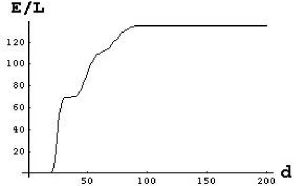
As a result of this, we obtain that the jump discontinuities in Figure 2 and Figure 3, will be smeared
out continuously over a large part of the interval. An example of this sort is presented in Figure 4
below.

included.
Figure 4
Fractions of Employment/Labor as a function
of traveling distance d to CBD
In Figure 4 we have assumed that Ψ is
defined in terms of a lognormal
distribution with mean $15 and with a
standard deviation of $3. Otherwise
the scenario is the same as in Figure 3.
Note the increase in values due to the
increase in traveling cost when time is
In reality a community will be equipped with a multitude of different goods and services, each with a
potentially different price reduction at the CBD. This puts our attention in the direction of
continuous distributions, in particular when we take into account such services with a flexible price,
e.g., paid according to the actual time spent on the service. Again we assume that all services have
been sorted in the direction of increased savings at the CBD. The density Φ Φ[pr] is defined in such
terms that the integral
More intriguing information
1. The name is absent2. A Unified Model For Developmental Robotics
3. Categorial Grammar and Discourse
4. An Empirical Analysis of the Curvature Factor of the Term Structure of Interest Rates
5. Howard Gardner : the myth of Multiple Intelligences
6. Nietzsche, immortality, singularity and eternal recurrence1
7. The changing face of Chicago: demographic trends in the 1990s
8. The name is absent
9. Who runs the IFIs?
10. The name is absent