subsequent analysis in which the additional inclusion of asset price variables might
strengthen the explanatory power of the global model.
Augmenting the VAR with asset prices
The next step in the VAR analysis is to allow for the first asset price variable to
enter the model. We start with the house price index (HPI), since - according to
section 3 - house prices may play a crucial role in this context. In the Cholesky
ordering, we put house prices just behind the GDP deflator, so that we are working
with the following vector of endogenous variables:
xt = (y p hpi IS m)t
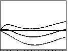
Response of Y to IS Response of P to IS Response of HPI to IS Response of M to IS
.006-
.004-
.002-
.000-
-.002-
-.004-
.006
.004
.002
.000
-.002
-.004
.012
.008
.004
.000
-.004
-.008
-.012
.008
.004
.000
-.004
-.008
Response of Y to M
Response of P to M
.006
.004
.002
.000
-.002
-.004
.012
-.008-
-.012
Response of HPI to M
Response of IS to M
.4-
.008
.004
.000
-.004
-.4-
2 4 6 8 10 12 14 16 18 20
2 4 6 8 10 12 14 16 18 20
2 4 6 8 10 12 14 16 18 20 2 4 6 8 10 12 14 16 18 20 2 4 6 8 10 12 14 16 18 20 2 4 6 8 10 12 14 16 18 20
.006-
.004-
.002-
.000-
-.002-
-.004-
2 4 6 8 10 12 14 16 18 20 2 4 6 8 10 12 14 16 18 20
Response of Y to HPI
4 6 8 10 12 14 16 18 20
Response of P to HPI
.006
.004
.002
.000
-.002
-.004

2 4 6 8 10 12 14 16 18 20
Response of IS to HPI Response of M to HPI
.4 --------------------------------------------------- .008--

-.2-∣ -.004-
-.4 .................. -.008 ..................
2 4 6 8 10 1 2 1 4 16 1 8 20 2 4 6 8 10 1 2 1 4 16 18 20
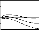
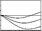
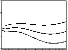
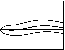
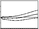
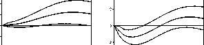
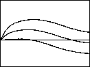
Figure 4: Impulse response analysis; basic model augmented with house prices
Figure 4 shows in the first row the effects from a positive shock to the short-
term interest rate. Like in the benchmark model, this kind of shock causes output
and money to decline, while the latter becomes significant at the 5% level here.
Moreover, the ”price puzzle” disappears which supports the view that house prices
19
More intriguing information
1. Spousal Labor Market Effects from Government Health Insurance: Evidence from a Veterans Affairs Expansion2. The name is absent
3. The name is absent
4. The name is absent
5. Individual tradable permit market and traffic congestion: An experimental study
6. Biological Control of Giant Reed (Arundo donax): Economic Aspects
7. The name is absent
8. ALTERNATIVE TRADE POLICIES
9. Empirically Analyzing the Impacts of U.S. Export Credit Programs on U.S. Agricultural Export Competitiveness
10. Stakeholder Activism, Managerial Entrenchment, and the Congruence of Interests between Shareholders and Stakeholders