|
Evo/Test |
1 |
2 |
3 |
4 |
5 |
6 |
7 |
8 |
|
Л |
1.02 (0.14) |
0.87 (0.1) |
1.45 (0.18) |
0.52 (0) |
1.26 (0.17) |
0.03 (0) |
0.2 (0.18) |
0.13 (0) |
|
2 |
0.28 (0.06) |
1.13 (0.35) |
0.18 (0.1) |
0.75 (0.26) |
0.5 (0.13) |
0.66 (0.19) |
0.18 (0.15) |
0.14 (0.02) |
|
3 |
0.58 (0.16) |
0.6 (0.22) |
2.1 (0.48) |
1.45 (0.66) |
0.62 (0.13) |
0.04 (0.1) |
0.03 (0.09) |
0.14 (0.02) |
|
4 |
0.15 (0.01) |
0.32 (0.02) |
0.06 (0.05) |
1.77 (0.52) |
0.22 (0.1) |
0.13 (0.13) |
0.07 (0.09) |
0.13 (0.02) |
|
5 |
0.07 (0.02) |
-0.02 (0) |
0.05 (0) |
0.2 (0.11) |
2.37 (0.28) |
0.1 (0.04) |
0.03 (0.05) |
0.13 (0.01) |
|
6 |
1.33 (0.18) |
0.43 (0.07) |
0.4 (0.2) |
0.67 (0.22) |
1.39 (0.42) |
2.34 (0.05) |
0.13 (0.13) |
0.14 (0.11) |
|
7 |
0.45 (0.11) |
0 (0.07) |
0.6 (0.18) |
0.03 (0.04) |
0.36 (0.08) |
0.07 (0.03) |
0.22 (0.15) |
0.08 (0) |
|
8__________ |
0.16 (0.03) |
0.28 (0.04) |
0.09 (0.07) |
0.29 (0.18) |
0.21 (0.03) |
0.08 (0.1) |
0.1 (0.09) |
0.13 (0) |
TABLE II
The fitness of each controller on each track. Each row represents the performance of the best controller of one
evolutionary run with fixed sensors, evolved the track with the same number as the row. Each column represents the
performance of the controllers on the track with the same number as the column. Each cell contains the mean fitness of 50
trials of the controller given by the row on the track given by the column. Cells with bold text indicate the track on which
A CERTAIN CONTROLLER PERFORMED BEST.
|
Track |
1 |
2 |
3 |
4 |
5 |
6 |
7 |
8 |
|
Fitness/sd |
1.66 (0.08) |
1.48 (0.25) |
2.56 (0.2) |
2.49 (0.15) |
2 (0.25) |
2.02 (0.42) ' |
0.4 (0.21) |
0.16 (0.07) ' |
TABLE IV
Fitnes s of an incrementally evolved general controller with fixed sensor parameters on the different tracks. Compound
FITNESS OVER ALL 8 TRACKS IS 2.01 (0.1 1).

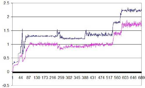
Fig. 3. A successful incremental run, producing a generally proficient
controller. New tracks were added to the fitness function when fitness of
the best controller reached 1.5; this happened at generations 53, 240, 253,
394 and 536. Maximum fitness continued to increase for approximately 50
generations after that. The graph show the fitness of the best controller (dark
line) and the mean fitness of the population.
because these runs suffer from ”premature specialization” -
after evolving a good controller for the first track, the sensor
setup might not be suited for good driving on the second
track, and changing the parameters would diminish fitness
on the first track, thus creating a local optimum. That the
first two tracks are, from the point of view of the car, mirror
images of each other, adds plausibility to this hypothesis.
C. Further evolution
Evolving sensor parameters can be beneficial, however,
when this is done for a controller that has already reached
general proficiency. We used one of the generally proficient

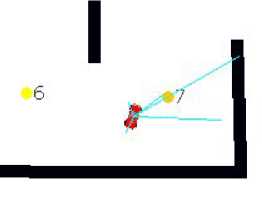
Fig. 4. Sensor setup of the further evolved general controller analysed in
table V. Only three sensors seem to be long enough to of any use, and
all of those point to the right or front-right. The asymmetry and ”waste”
is somewhat surprising, as the controller performs well on all the first six
tracks (but it does do slightly better on clockwise than on anti-clockwise
tracks).
controllers evolved using the incremental method as the seed
for a new evolutionary run, with sensor mutation turned
on and controllers tested on all six tracks simultaneously.
The results was an increase in mean fitness, as can be seen
in V. Although the mean fitness does not increase on every
single track, the best controller of the last generation races
all the tracks more reliably, and is very rarely observed to
crash into a wall in such a way that the car gets stuck. The
evolved sensors of this controller showed little similiarity to
the original sensor setup, described above - see figure 4 for
an example.
VI. Evolving specialized controllers
In order to see whether we could create even better
controllers, we used one of the further evolved controllers
(with evolved sensor parameters) as basis for specializing
More intriguing information
1. The name is absent2. The name is absent
3. The name is absent
4. Gerontocracy in Motion? – European Cross-Country Evidence on the Labor Market Consequences of Population Ageing
5. LOCAL CONTROL AND IMPROVEMENT OF COMMUNITY SERVICE
6. The name is absent
7. Auction Design without Commitment
8. Language discrimination by human newborns and by cotton-top tamarin monkeys
9. Measuring Semantic Similarity by Latent Relational Analysis
10. The Social Context as a Determinant of Teacher Motivational Strategies in Physical Education