Inflation and Inflation Uncertainty in the Euro Area

In all cases we conclude that there is time variation, either in the form of non-
stationarity or in the form of structural breaks, which justifies the use of time-varying
parameters in the AR equation. Similarly, we test for the significance of the ARCH
and GARCH parameters of the model, finding that they are both significant. We
report in Table 1 the Ljung-Box test statistic for serial correlation of the residuals at
lags 1 to 4, showing that there is no residual autocorrelation at 5% level.

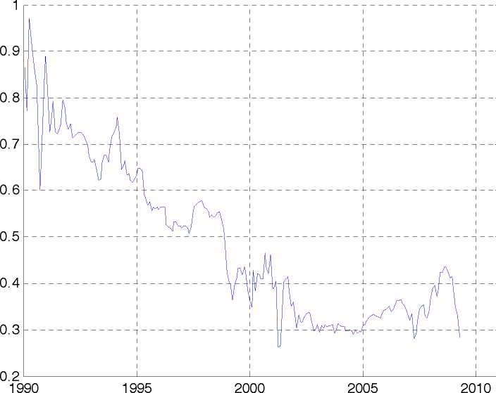
Charts 4-9 are based on the estimation results. Chart 4 shows trend inflation, namely
the estimated time-varying constant from Equation (4), which declines steadily from
the beginning of the 1990s up to the start of EMU, stabilising afterwards. The
estimates of the individual coefficients on lagged unemployment (not reported) are
not particularly informative, but it is clear that their sum, shown in Chart 5, is
negative throughout the sample. This is consistent with our earlier interpretation of
the data based on the Phillips curve model. It suggests again that this curve has
become flatter since the introduction of the euro, possibly reflecting a more firm
anchoring of inflation expectations.

Chart 4. EMU Trend inflation (month on month)

Chart 6 plots inflation persistence, defined as the sum of its autoregressive
coefficients. This exhibits a positive trend becoming negative at the beginning of the
third Phase of EMU, which may reflect lower and better-anchored inflation
expectations in the post-1999 period, consistently with the ECB’s mandate of
achieving long-term price stability and with theory. For instance, Erceg and Levin
(2003) show that inflation displays very little persistence if the long-run inflation
target is constant. Similarly, Orphanides and Williams (2005) demonstrate that if
long-run inflation expectations are well anchored, then inflation will be less persistent
than if the public is uncertain about the long-run inflation target.

<<   8   9   10   11   12   13   14   >>

More intriguing information